covariance_matrix

detkit.covariance_matrix(size=512, sample=2, cor=False, ecg_start=0.0, ecg_end=30.0, ecg_wrap=True, plot=False, verbose=False)

Create covariance matrix based on the autocorrelation of electrocardiogram signal.

Parameters:

sizeint, default=2**9

Size of the matrix.

sampleint, default=2

Sampling pace of the autocorrelation function.

corbool, default=False

If True, instead of the covariance matrix, the correlation matrix is returned.

ecg_startfloat, default=0.0

Start time of the electrocardiogram signal in seconds.

ecg_endfloat, default=30.0

End time of the electrocardiogram signal in seconds.

ecg_wrapbool, default=True

If True, the electrocardiogram signal is assumed to be wrapped.

plotbool or str, default=False

If True, the covariance matrix is plotted. If plot is a string, the plot is not shown, rather saved with a filename as the given string. If the filename does not contain file extension, the plot is saved in both svg and pdf formats. If the filename does not have directory path, the plot is saved in the current directory.

verbosebool, default=False

if True, the saved plot filename is printed.

Returns:

matrixnumpy.ndarray

The covariance (or correlation, if cor is True) matrix.

See also

detkit.electrocardiogram

detkit.design_matrix

Notes

Autocorrelation Function:

The covariance matrix is computed based on the autocorrelation of and ECG signal. It is assumed that the ECG signal is wide-sense stationary stochastic process, so its autocovariance function can be defined by

\[\kappa(\Delta t) = \mathbb{E}[ (f(t+\Delta t) - \bar{f})(f(t) - \bar{f})],\]

where \(f\) is the ECG signal, \(\Delta t\) is the lag-time of the autocorrelation function, \(\mathbb{E}\) is the expectation operator, and \(\bar{f}\) is the mean of the \(f\). The autocorrelation function is defined by

\[\tau(\Delta t) = \sigma^{-2} \kappa(\Delta t),\]

where \(\sigma^2 = \kappa(0)\) is the variance of the ECG signal.

Covariance Matrix:

The covariance matrix \(\boldsymbol{\Sigma}\) is defined by its \(i,j\) components as

\[\Sigma_{ij} = \kappa(\vert i - j \vert f_s \nu)\]

where \(f_s = 360\) Hz is the sampling frequency of the ECG signal and \(\nu\) is the sampling of the autocorrelation function that is specified by sample argument.

The total time span of the correlation matrix is

\[\Delta t = n \frac{\nu}{f_s},\]

where \(n\) is the size of the matrix.

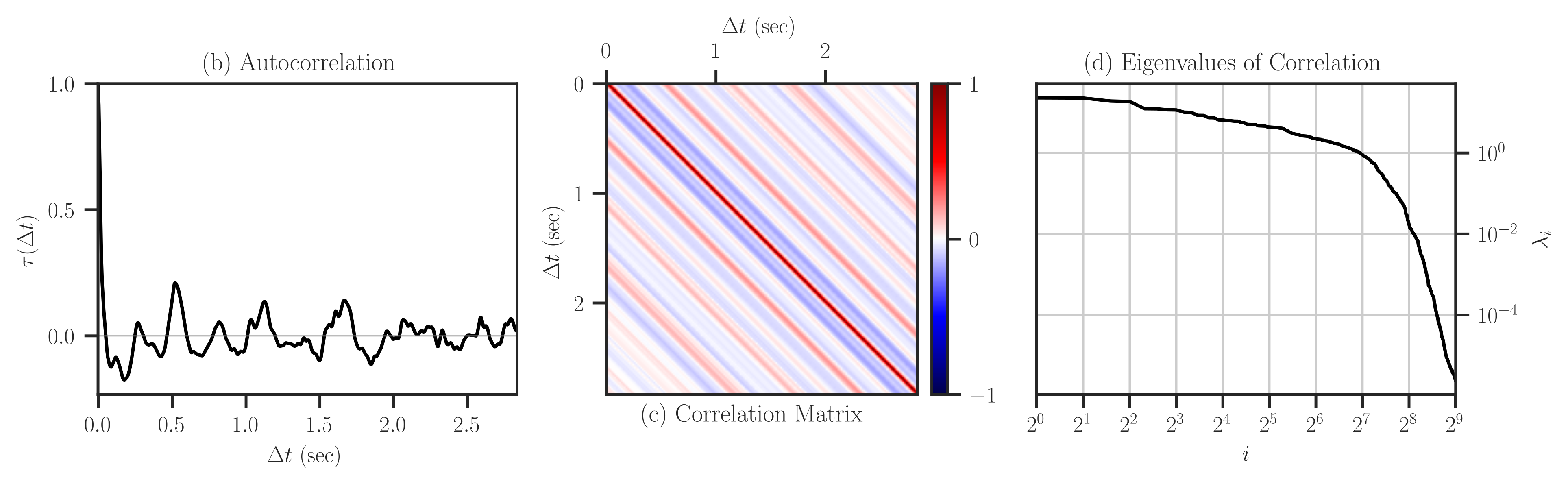
For instance, for the matrix size 2**9 and sampling 2, the matrix spans 2.84 seconds.

Correlation versus Covariance:

If cor is True, the correlation matrix is instead computed and plotted. The covariance matrix \(\boldsymbol{\Sigma}\) is a scalar multiple of the correlation matrix \(\mathbf{K}\) by

\[\mathbf{K} = \sigma^{-2} \boldsymbol{\Sigma}.\]

Examples

>>> from detit.datasets import covariance_matrix
>>> A = covariance_matrix(size=2**9, cor=True, plot=True)