imate.eigencount(method=’slq’)#
- imate.eigencount(A, gram=False, p=1.0, interval=[0.0, 1.0], return_info=False, method='slq', parameters=None, min_num_samples=10, max_num_samples=50, error_atol=None, error_rtol=0.01, confidence_level=0.95, outlier_significance_level=0.001, lanczos_degree=20, lanczos_tol=None, orthogonalize=0, seed=None, num_threads=0, num_gpu_devices=0, gpu=False, verbose=False, plot=False)
See also
This page describes only the slq method. For other methods, see
imate.eigencount().Eigencount of matrix or linear operator using eigenvalue method.
Given the symmetric matrix or linear operator \(\mathbf{A}\) and the real exponent \(p\), the following is computed:
\[\mathrm{trace} f \left(\mathbf{A}^p \right),\]\[f(\lambda) = \mathbb{1}_{[\lambda_{\min}, \lambda_{\max}]}(\lambda),\]where \(\mathbb{1}_{[\lambda_{\min}, \lambda_{\max}]}(\lambda)\) is the indicator function in the interval \([\lambda_{\min}, \lambda_{\max}]\). The above trace effectively counts the number of eigenvalues of the matrix in a specified interval.
If
gramis True, then \(\mathbf{A}\) in the above is replaced by the Gramian matrix \(\mathbf{A}^{\intercal} \mathbf{A}\), and the following is instead computed:\[\mathrm{trace} f \left((\mathbf{A}^{\intercal}\mathbf{A})^p \right).\]If \(\mathbf{A} = \mathbf{A}(t)\) is a linear operator of the class
imate.AffineMatrixFunctionwith the parameter \(t\), then for an input tuple \(t = (t_1, \dots, t_q)\), an array output of the size \(q\) is returned, namely:\[\mathrm{trace} f \left((\mathbf{A}(t_i))^p \right), \quad i=1, \dots, q.\]- Parameters:
- Anumpy.ndarray, scipy.sparse,
imate.Matrix, orimate.AffineMatrixFunction A sparse or dense matrix or linear operator. If
gramis False, then A should be symmetric.Warning
The symmetry of A is not pre-checked by this function. If
gramis False, make sure A is symmetric.- grambool, default=False
If True, the log-determinant of the Gramian matrix, \((\mathbf{A}^{\intercal}\mathbf{A})^p\), is computed. The Gramian matrix itself is not directly computed. If False, the log-determinant of \(\mathbf{A}^p\) is computed.
- pfloat, default=1.0
The real exponent \(p\) in \(\mathbf{A}^p\).
- interval(tuple, list, numpy.array), default=[0.0, 1.0]
A list of two float numbers representing the minimum and maximum eigenvalues \(\lambda_{\min}\) and \(\lambda_{\max}\), respectively.
- return_infobool, default=False
If True, this function also returns a dictionary containing information about the inner computation, such as process time, algorithm settings, etc.
- parametersarray_like [float], default=one
This argument is relevant if A is a type of
AffineMatrixFunction. By this argument, multiple inquiries, \((t_1, \dots, t_q)\), can be passed to the parameter \(t\) of the linear operator \(\mathbf{A}(t)\). The output of this function becomes an array of the size \(q\) corresponding to each of the input matrices \(\mathbf{A}(t_i)\).- min_num_samplesint, default=10
The minimum number of Monte-Carlo samples. If the convergence criterion is reached before finishing the minimum number of iterations, the iterations are forced to continue till the minimum number of iterations is finished. This value should be smaller than
maximum_num_samples.- max_num_samplesint, default=50
The maximum number of Monte-Carlo samples. If the convergence criterion is not reached by the maximum number of iterations, the iterations are forced to stop. This value should be larger than
minimum_num_samples.- error_atolfloat, default=None
Tolerance of the absolute error of convergence of the output. Once the error of convergence reaches
error_atol + error_rtol * output, the iteration is terminated. If the convergence criterion is not met by the tolerance, then the iterations continue till reachingmax_num_samplesiterations. If None, the termination criterion does not depend on this parameter.- error_rtolfloat, default=None
Tolerance of the relative error of convergence of the output. Once the error of convergence reaches
error_atol + error_rtol * output, the iteration is terminated. If the convergence criterion is not met by the tolerance, then the iterations continue till reachingmax_num_samplesiterations. If None, the termination criterion does not depend on this parameter.- confidence_levelfloat, default=0.95
Confidence level of error, which is a number between 0 and 1. The error of convergence of the population of samples is defined by their standard deviation times the Z-score, which depends on the confidence level. See notes below for details.
- outlier_significance_levelfloat, default=0.001
One minus the confidence level of the uncertainty of the outliers of the output samples. This is a number between 0 and 1.
- lanczos_degreeint, default=20
The number of Lanczos recursive iterations. The larger Lanczos degree leads to better estimation. The computational cost quadratically increases with the Lanczos degree.
- lanczos_tolfloat, default=None
The tolerance to stop the Lanczos recursive iterations before the end of iterations reached. If the tolerance is not met, all the iterations (total of
lanczos_degreeiterations) continue till the end. If set to None (default value), the machine’ epsilon precision is used. The machine’s epsilon precision is as follows:For 32-bit, machine precision is \(2^{-23} = 1.1920929 \times 10^{-7}\).
For 64-bit, machine precision is \(2^{-52} = 2.220446049250313 \times 10^{-16}\),
For 128-bit, machine precision is \(2^{-63} = -1.084202172485504434 \times 10^{-19}\).
- orthogonalizeint, default=0
Indicates whether to re-orthogonalize the eigenvectors during Lanczos recursive iterations.
If set to 0, no orthogonalization is performed.
If set to a negative integer or an integer larger than
lanczos_degree, a newly computed eigenvector is orthogonalized against all the previous eigenvectors (also known as full reorthogonalization).If set to a positive integer, say q, but less than
lanczos_degree, the newly computed eigenvector is orthogonalized against a window of last q previous eigenvectors (known as partial reorthogonalization).
- seedint, default=None
A non-negative integer that serves as the seed for generating sequences of pseudo-random numbers within the algorithm. This parameter allows you to control the randomness and make the results of the randomized algorithm reproducible.
If
seedis set toNoneor a negative integer, the provided seed value is ignored, and the algorithm uses the current processor time as the seed. As a result, the generated sequences are pseudo-random, and the outcome is not reproducible.Note
For reproducibility, it’s essential not only to specify the
seedparameter as a non-negative integer but also to setnum_threadsto1.- num_threadsint, default=0
Number of processor threads to employ for parallel computation on CPU. If set to 0 or a number larger than the available number of threads, all threads of the processor are used. The parallelization is performed over the Monte-Carlo iterations.
- num_gpu_devicesint default=0
Number of GPU devices (if available) to use for parallel multi-GPU processing. If set to 0, the maximum number of available GPU devices is used. This parameter is relevant if
gpuis True.- gpubool, default=False
If True, the computations are performed on GPU devices where the number of devices can be set by
num_gpu_devices. If no GPU device is found, it raises an error.Note
When performing repetitive computation on the same matrix on GPU, it is recommended to input A as an instance of
imate.Matrixclass instead of numpy or scipy matrices. See examples below for clarification.- verbosebool, default=False
Prints extra information about the computations.
- plotbool or str, default=False
If True, convergence of samples will be plotted. If no graphical backend is available (such as executing on remote machines) the plot is instead saved in the current directory as both
svgandpdfformat. Ifplotis a string, the plot is not shown, rather saved with a filename as the given string. If the filename does not contain file extension, the plot is saved in bothsvgandpdfformats. If the filename does not have directory path, the plot is saved in the current directory.
- Anumpy.ndarray, scipy.sparse,
- Returns:
- trlinexpfloat or numpy.array
Log-determinant of A. If A is of type
imate.AffineMatrixFunctionwith an array ofparameters, then the output is an array.- infodict
(Only if
return_infois True) A dictionary of information with the following.matrix:data_type: str, {float32, float64, float128}. Type of the matrix data.gram: bool, whether the matrix A or its Gramian is considered.exponent: float, the exponent p in \(\mathbf{A}^p\).size: (int, int) The size of matrix A.sparse: bool, whether the matrix A is sparse or dense.nnz: int, if A is sparse, the number of non-zero elements of A.density: float, if A is sparse, the density of A, which is the nnz divided by size squared.num_inquiries: int, the size of inquiries of each parameter of the linear operator A. If A is a matrix, this is always 1. If A is a type ofAffineMatrixFunction, this value is the number of \(t_i\) parameters.num_operator_parameters: int, number of parameters of the operator A. If A a type ofAffineMatrixFunction, then this value is 1 corresponding to one parameter \(t\) in the affine function t mapsto mathbf{A} + t mathbf{B}.parameters: list [float], the parameters of the linear operator A.
convergence:all_converged: bool, whether the Monte-Carlo sampling converged for all requested parameters \(t_i\). If all entries of the array forconvergedis True`, then this value is alsoTrue.converged: array [bool], whether the Monte-Carlo sampling converged for each of the requested parameters \(t_i\). Convergence is defined based on a termination criterion, such as absolute or relative error. If the iterations terminated due to reaching the maximum number of samples, this value is False.min_num_samples: int, the minimum number of Monte-Carlo iterations.max_num_samples: int, the maximum number of Monte-Carlo iterations.num_outliers: int, number of outliers found during search for outliers among the array of output.num_samples_used: int, number of Monte-Carlo samples used to produce the output. This is the total number of iterations minus the number of outliers.samples: array [float], an array of the size max_num_samples. The first few entries (num_samples_used) of this array are the output results of the Monte-Carlo sampling. The average of these samples is the final result. The rest of this array is nan.samples_mean: float, mean of the samples array, excluding the nan values.samples_processed_order: array [int], in parallel processing, samples are processed in non-sequential order. This array, which has the same size as samples, keeps track of the order in which each sample is processed.
error:absolute_error: float, the absolute error of the convergence of samples.confidence_level: float, the confidence level used to calculate the error from standard deviation of samples.error_atol: float, the tolerance of absolute error of the convergence of samples.error_rtol: float, the tolerance of relative error of the convergence of samples.outlier_significance_level: float, the significance level used to determine the outliers in samples.relative_error: float, the relative error of the convergence of samples.
device:num_cpu_threads: int, number of CPU threads used in shared memory parallel processing.num_gpu_devices: int, number of GPU devices used in the multi-GPU (GPU farm) computation.num_gpu_multiprocessors: int, number of GPU multi-processors.num_gpu_threads_per_multiprocessor: int, number of GPU threads on each GPU multi-processor.
time:tot_wall_time: float, total elapsed time of computation.alg_wall_time: float, elapsed time of computation during only the algorithm execution.cpu_proc_time: float, the CPU processing time of computation.
solver:version: str, version of imate.method: ‘slq’.lanczos_degree: bool, Lanczos degree.lanczos_tol: float, Lanczos tolerance.orthogonalize: int, orthogonalization flag.seed: int, seed value for random number generation.
- Raises:
- ImportError
If the package has not been compiled with GPU support, but
gpuis set to True. To resolve the issue, setgputo False to be able to use the existing installation. Alternatively, export the environment variableUSE_CUDA=1and recompile the source code of the package.
Notes
Computational Complexity:
This method uses stochastic Lanczos quadrature (SLQ), which is a randomized algorithm. The computational complexity of this method is
\[\mathcal{O}((\rho n^2 + n l) s l),\]where \(n\) is the matrix size, \(\rho\) is the density of sparse matrix (for dense matrix, \(\rho=1\)), \(l\) is the Lanczos degree (set with
lanczos_degree), and \(s\) is the number of samples (set withmin_num_samplesandmax_num_samples).This method can be used on very large matrices (\(n > 2^{12}\)). The solution is an approximation.
Input Matrix:
The input A can be either of:
A matrix, such as numpy.ndarray, or scipy.sparse.
A linear operator representing a matrix using
imate.Matrix.A linear operator representing a one-parameter family of an affine matrix function \(t \mapsto \mathbf{A} + t\mathbf{B}\) using
imate.AffineMatrixFunction.
Output:
The output is a scalar. However, if A is the linear operator \(\mathbf{A}(t) = \mathbf{A} + t \mathbf{B}\) where \(t\) is given as the tuple \(t = (t_1, \dots, t_q)\), then the output of this function is an array of size \(q\) corresponding to the race-exponential of each \(\mathbf{A}(t_i)\).
Note
When A represents \(\mathbf{A}(t) = \mathbf{A} + t \mathbf{I}\), where \(\mathbf{I}\) is the identity matrix, and \(t\) is given by a tuple \(t = (t_1, \dots, t_q)\), the computational cost of an array output of size q is the same as computing for a single \(t_i\). Namely, the trace-exponential of only \(\mathbf{A}(t_1)\) is computed, and the trace-exponential of the rest of \(i=2, \dots, q\) are obtained from the result of \(t_1\) immediately.
Algorithm:
If
gramis False, the Lanczos tri-diagonalization method is used. This method requires only matrix-vector multiplication. Ifgramis True, the Golub-Kahn bi-diagonalization method is used. This method requires both matrix-vector multiplication and transposed-matrix vector multiplications.Convergence criterion:
Let \(n_{\min}\) and \(n_{\max}\) be the minimum and maximum number of iterations respectively defined by
min_num_samplesandmax_num_samples. The iterations terminate at \(n_{\min} \leq i \leq n_{\max}\) where \(i\) is the iteration counter. The iterations stop earlier at \(i < n_{\max}\) if the convergence error of the mean of the samples is satisfied, as follows.Suppose \(s(j)\) and \(\sigma(i)\) are respectively the mean and standard deviation of samples after \(j\) iterations. The error of convergence, \(e(j)\), is defined by
\[e(j) = \frac{\sigma(j)}{\sqrt{j}} Z\]where \(Z\) is the Z-score defined by
\[Z = \sqrt{2} \mathrm{erf}^{-1}(\phi).\]In the above, \(\phi\) is the confidence level and set by
confidence_levelargument, and \(\mathrm{erf}^{-1}\) is the inverse error function. A confidence level of 95%, for instance, means that the Z-score is 1.96, which means the confidence interval is \(\pm 1.96 \sigma\).The termination criterion is
\[e(j) < \epsilon_a + s(j) \epsilon_r,\]where \(\epsilon_{a}\) and \(\epsilon_r\) are the absolute and relative error tolerances respectively, and they are set by
error_atolanderror_rtol.Convergence for the case of multiple parameters:
When A is a type of
imate.AffineMatrixFunctionrepresenting the affine matrix function \(\mathbf{A}(t) = \mathbf{A} + t \mathbf{B}\) and if multiple parameters \(t_i\), \(i=1,\dots, q\) are passed to this function throughparametersargument, the convergence criterion has to be satisfied for each of \(\mathbf{A}(t_i)\). Specifically, the iterations are terminated as follows:If \(\mathbf{B}\) is the identity matrix, iterations for all \(\mathbf{A}(t_i)\) continue till the convergence criterion for all \(t_i\) are satisfied. That is, even if \(t=t_i\) is converged but \(t=t_j\) has not converged yet, the iterations for \(t=t_i\) will continue. :
If \(\mathbf{B}\) is not the identity matrix, the iterations for each of \(t_i\) are independent. That is, if \(t=t_i\) converges, the iterations for that parameter will stop regardless of the convergence status of other parameters.
Plotting:
If
plotis set to True, it plots the convergence of samples and their relative error.If no graphical backend exists (such as running the code on a remote server or manually disabling the X11 backend), the plot will not be shown, rather, it will be saved as an
svgfile in the current directory.If the executable
latexis available onPATH, the plot is rendered using \(\rm\LaTeX\) and it may take slightly longer to produce the plot.If \(\rm\LaTeX\) is not installed, it uses any available San-Serif font to render the plot.
To manually disable interactive plot display and save the plot as
svginstead, add the following at the very beginning of your code before importingimate:>>> import os >>> os.environ['IMATE_NO_DISPLAY'] = 'True'
References
Ubaru, S., Chen, J., and Saad, Y. (2017), Fast Estimation of \(\mathrm{tr}(F(A))\) Via Stochastic Lanczos Quadrature, SIAM J. Matrix Anal. Appl., 38(4), 1075-1099.
Examples
Symmetric Input Matrix:
The slq method requires the input matrix of
imate.eigencount()function to be symmetric whengramis False. For the first example, generate a symmetric sample matrix usingimate.toeplitz()function as follows:>>> # Import packages >>> from imate import toeplitz >>> # Generate a symmetric matrix by setting gram=True. >>> A = toeplitz(2, 1, size=100, gram=True)
In the above, by passing
gram=Truetoimate.toeplitz()function, the Gramian of the Toeplitz matrix is returned, which is symmetric. Compute the race-exponential of \(\mathbf{A}^{2.5}\):>>> # Import packages >>> from imate import eigencount >>> # Compute the trace-exponential >>> eigencount(A, gram=False, p=2.5, method='slq') 277.00578301560057
Gramian Matrix:
Passing
gram=Truetoimate.eigencount()function uses the Gramian of the input matrix. n this case, the input matrix can be non-symmetric. In the next example, generate a non-symmetric matrix, \(\mathbf{B}\), then compute the trace-exponential of \((\mathbf{B}^{\intercal} \mathbf{B})^{2.5}\).>>> # Generate a non-symmetric matrix by setting gram=False >>> B = toeplitz(2, 1, size=100, gram=False) >>> # Compute trace-exponential of Gramian by passing gram=True >>> eigencount(B, gram=True, p=2.5, method='slq') 275.15518680196476
Note that the result of the two examples in the above are the similar since the input matrix \(\mathbf{A}\) of the first example is the Gramian of the input matrix \(\mathbf{B}\) in the second example, that is \(\mathbf{A} = \mathbf{B}^{\intercal} \mathbf{B}\). Since the second example uses the Gramian of the input matrix, it computes the same quantity as the first example.
Verbose output:
By setting
verboseto True, useful info about the process is printed.>>> ld = logdet(A, method='slq', verbose=True) results ============================================================================== inquiries error samples -------------------- --------------------- --------- i parameters trace absolute relative num out converged ============================================================================== 1 none +1.386e+06 8.218e+02 0.059% 10 0 True config ============================================================================== matrix stochastic estimator ------------------------------------- ------------------------------------- gram: False method: slq exponent: 1 lanczos degree: 20 num matrix parameters: 0 lanczos tol: 2.220e-16 data type: 64-bit orthogonalization: none convergence error ------------------------------------- ------------------------------------- min num samples: 10 abs error tol: 0.000e+00 max num samples: 50 rel error tol: 1.00% outlier significance level: 0.00% confidence level: 95.00% process ============================================================================== time device ------------------------------------- ------------------------------------- tot wall time (sec): 2.609e+00 num cpu threads: 8 alg wall time (sec): 2.605e+00 num gpu devices, multiproc: 0, 0 cpu proc time (sec): 1.798e+01 num gpu threads per multiproc: 0
Output information:
Print information about the inner computation:
>>> ld, info = eigencount(A, method='slq', return_info=True)
>>> print(ld)
138.6294361119891

>>> # Print dictionary neatly using pprint
>>> from pprint import pprint
>>> pprint(info)
{
    'matrix': {
        'data_type': b'float64',
        'density': 0.0298,
        'exponent': 1.0,
        'gram': False,
        'nnz': 298,
        'num_inquiries': 1,
        'num_operator_parameters': 0,
        'parameters': None,
        'size': (100, 100),
        'sparse': True
    },
    'convergence': {
        'all_converged': False,
        'converged': False,
        'max_num_samples': 50,
        'min_num_samples': 10,
        'num_outliers': 0,
        'num_samples_used': 50,
        'samples': array([124.65021242, ..., 143.27314446]),
        'samples_mean': 139.89509513079338,
        'samples_processed_order': array([ 4, ..., 47])
    },
    'error': {
        'absolute_error': 2.345203485787551,
       'confidence_level': 0.95,
       'error_atol': 0.0,
       'error_rtol': 0.01,
       'outlier_significance_level': 0.001,
       'relative_error': 0.01676401508998531
    },
    'solver': {
        'lanczos_degree': 20,
        'lanczos_tol': 2.220446049250313e-16,
        'method': 'slq',
        'orthogonalize': 0,
        'seed': None,
        'version': '0.15.0'
    },
    'device': {
        'num_cpu_threads': 8,
        'num_gpu_devices': 0,
        'num_gpu_multiprocessors': 0,
        'num_gpu_threads_per_multiprocessor': 0
    },
    'time': {
        'alg_wall_time': 0.002254009246826172,
        'cpu_proc_time': 0.01330678200000035,
        'tot_wall_time': 0.0023698790464550257
    }
}
Large matrix:
Compute the trace-exponential of a very large sparse matrix using at least 100 samples:
>>> # Generate a matrix of size one million
>>> A = toeplitz(2, 1, size=1000000, gram=True)

>>> # Approximate trace-exponential using stochastic Lanczos quadrature
>>> # with at least 100 Monte-Carlo sampling
>>> ld, info = eigencount(A, method='slq', min_num_samples=100,
...                  max_num_samples=200, return_info=True)
>>> print(ld)
1386320.4734751645

>>> # Find the time it took to compute the above
>>> print(info['time'])
{
    'tot_wall_time': 16.598053652094677,
    'alg_wall_time': 16.57977867126465,
    'cpu_proc_time': 113.03275911399999
}
Plotting:
By setting
plotto True, plots of samples during Monte-Carlo iterations and the convergence of their mean are generated.>>> A = toeplitz(2, 1, size=1000000, gram=True) >>> eigencount(A, method='slq', min_num_samples=20, max_num_samples=80, ... error_rtol=2e-4, confidence_level=0.95, ... outlier_significance_level=0.001, plot=True)
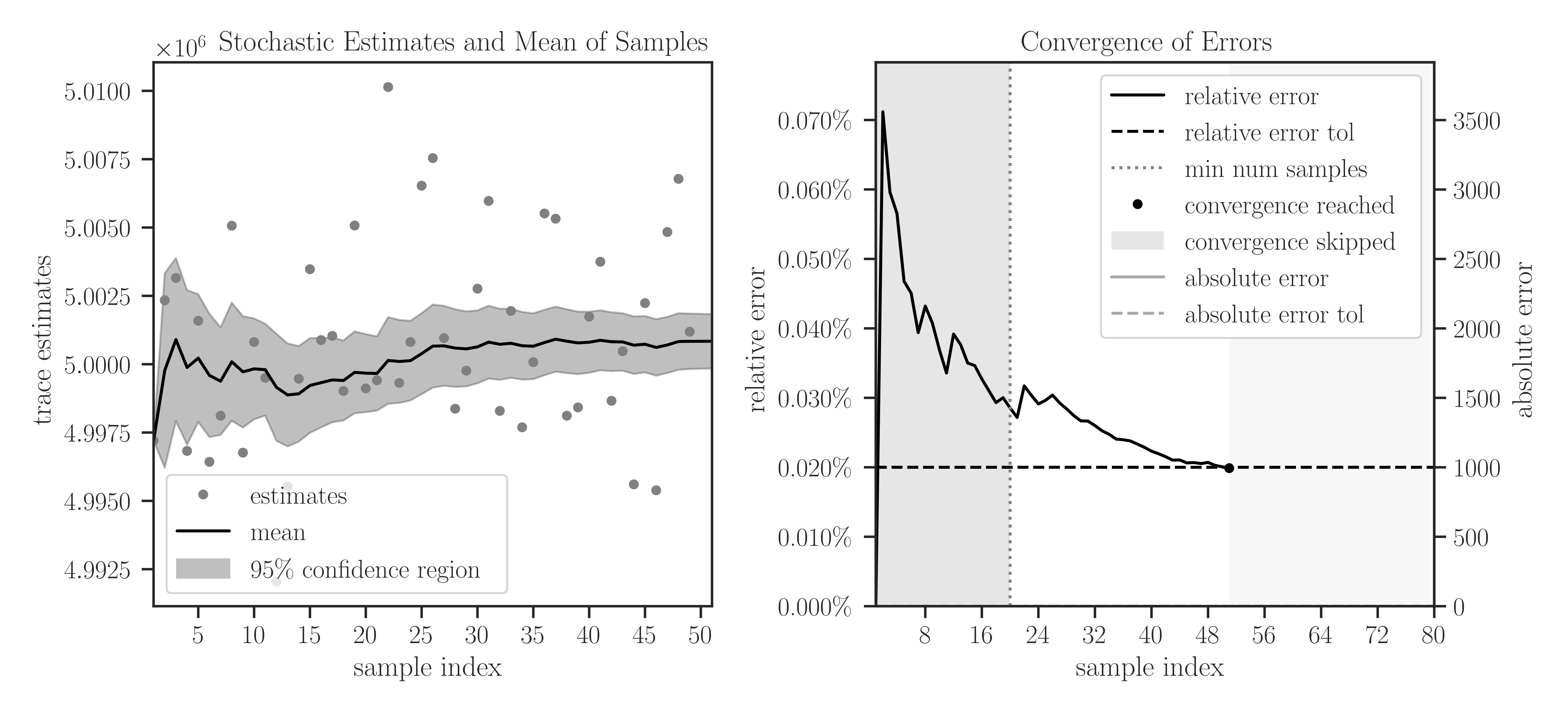
In the left plot, the samples are shown in circles and the cumulative mean of the samples is shown by a solid black curve. The shaded area corresponds to the 95% confidence interval \(\pm 1.96 \sigma\), which is set by
confidence_level=0.95. The samples outside the interval of 99.9% are considered outliers, which is set by the significance leveloutlier_significance_level=0.001.In the right plot, the darker shaded area in the interval \([0, 20]\) shows the minimum number of samples and is set by
min_num_samples=20. The iterations do not stop till the minimum number of iterations is passed. We can observe that sampling is terminated after 55 iterations where the relative error of samples reaches 0.02% since we seterror_rtol=2e-4. The lighter shaded area in the interval \([56, 80]\) corresponds to the iterations that were not performed to reach the specified maximum iterations bymax_num_samples=80.Matrix operator:
Use an object of
imate.Matrixclass as an alternative method to pass the matrix A to the eigencount function.>>> # Import matrix operator >>> from imate import toeplitz, eigencount, Matrix >>> # Generate a sample matrix (a toeplitz matrix) >>> A = toeplitz(2, 1, size=100, gram=True) >>> # Create a matrix operator object from matrix A >>> Aop = Matrix(A) >>> # Compute trace-exponential of Aop >>> eigencount(Aop, method='slq') 141.52929878934194
An advantage of passing Aop (instead of A) to the eigencount function will be clear when using GPU.
Computation on GPU:
The argument
gpu=Trueperforms the computations on GPU. The following example uses the object Aop created earlier.>>> # Compute trace-exponential of Aop >>> eigencount(Aop, method='slq', gpu=True) 141.52929878934194
The above function call triggers the object Aop to automatically load the matrix data on the GPU.
One could have used A instead of Aop in the above. However, an advantage of using Aop (instead of the matrix A directly) is that by calling the above eigencount function (or another function) again on this matrix, the data of this matrix does not have to be re-allocated on the GPU device again. To highlight this point, call the above function again, but this time, set
gramto True to compute something different.>>> # Compute trace-exponential of Aop >>> eigencount(Aop, method='slq', gpu=True, gram=True) 141.52929878934194
In the above example, no data is needed to be transferred from CPU host to GPU device again. However, if A was used instead of Aop, the data would have been transferred from CPU to GPU again for the second time. The Aop object holds the data on GPU for later use as long as this object does no go out of the scope of the python environment. Once the variable Aop goes out of scope, the matrix data on all the GPU devices will be cleaned automatically.
Affine matrix operator:
Use an object of
imate.AffineMatrixFunctionto create the linear operator\[\mathbf{A}(t) = \mathbf{A} + t \mathbf{I}.\]The object \(\mathbf{A}(t)\) can be passed to eigencount function with multiple values for the parameter \(t\) to compute their trace-exponential all at once, as follows.
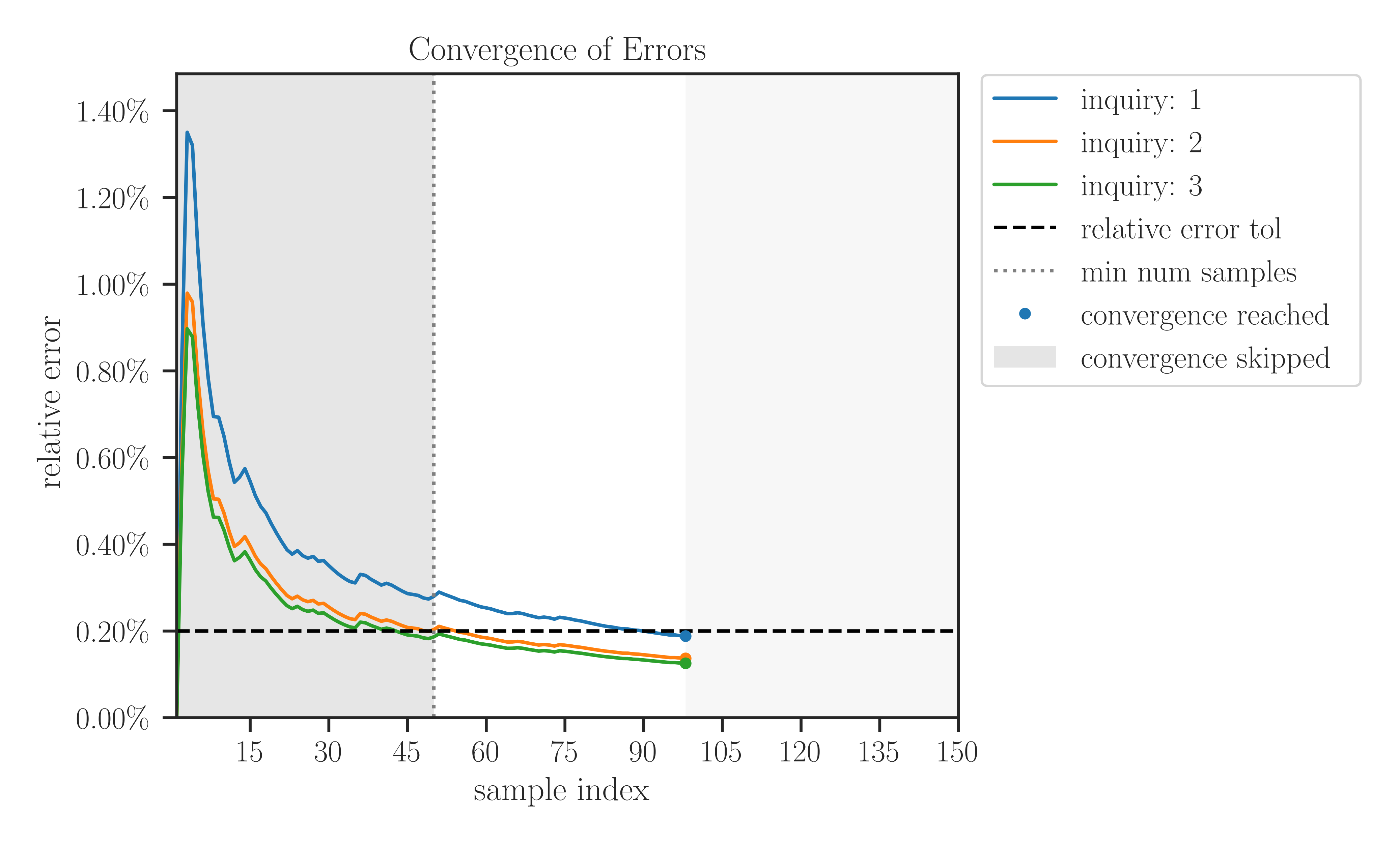
>>> # Import affine matrix function
>>> from imate import toeplitz, eigencount, AffineMatrixFunction

>>> # Generate a sample matrix (a toeplitz matrix)
>>> A = toeplitz(2, 1, size=100, gram=True)

>>> # Create a matrix operator object from matrix A
>>> Aop = AffineMatrixFunction(A)

>>> # A list of parameters t to pass to Aop
>>> t = [-1.0, 0.0, 1.0]

>>> # Compute trace-exponential of Aop for all parameters t
>>> eigencount(Aop, method='slq', parameters=t, min_num_samples=20,
...       max_num_samples=80, error_rtol=1e-3, confidence_level=0.95,
...       outlier_significance_level=0.001, plot=True, verbose=True)
array([ 68.71411681, 135.88356906, 163.44156683])
The output of the verbose argument is shown below. In the results section of the table below, each row i under the inquiry column corresponds to each element of the parameters
t = [-1, 0, 1]that was specified byparametersargument.results ============================================================================== inquiries error samples -------------------- --------------------- --------- i parameters trace absolute relative num out converged ============================================================================== 1 -1.0000e+00 +7.277e+05 6.748e+02 0.093% 39 0 True 2 0.0000e+00 +1.386e+06 2.947e+02 0.021% 39 0 True 3 1.0000e+00 +1.656e+06 2.231e+02 0.013% 39 0 True config ============================================================================== matrix stochastic estimator ------------------------------------- ------------------------------------- gram: False method: slq exponent: 1 lanczos degree: 20 num matrix parameters: 1 lanczos tol: 2.220e-16 data type: 64-bit orthogonalization: none convergence error ------------------------------------- ------------------------------------- min num samples: 20 abs error tol: 0.000e+00 max num samples: 80 rel error tol: 0.10% outlier significance level: 0.00% confidence level: 95.00% process ============================================================================== time device ------------------------------------- ------------------------------------- tot wall time (sec): 7.034e+00 num cpu threads: 8 alg wall time (sec): 7.031e+00 num gpu devices, multiproc: 0, 0 cpu proc time (sec): 4.895e+01 num gpu threads per multiproc: 0
The output of the plot is shown below. Each colored curve corresponds to a parameter in
t = [-1, 0, 1].