imate.InterpolateSchatten(kind=’crf’)#

class imate.InterpolateSchatten(A, B=None, p=0, options={}, verbose=False, ti=[], kind='crf', scale=None, func_type=1)

Interpolate Schatten norm (or anti-norm) of an affine matrix function using Chebyshev rational functions (CRF) method.

See also

This page describes only the crf method. For other kinds, see imate.InterpolateSchatten().

Parameters:

Anumpy.ndarray, scipy.sparse matrix

Symmetric positive-definite matrix (positive-definite if p is non-positive). Matrix can be dense or sparse.

Warning

Symmetry and positive (semi-) definiteness of A will not be checked. Make sure A satisfies these conditions.

Bnumpy.ndarray, scipy.sparse matrix, default=None

Symmetric positive-definite matrix (positive-definite if p is non-positive). Matrix can be dense or sparse. B should have the same size and type of A. If B is None (default value), it is assumed that B is the identity matrix.

Warning

Symmetry and positive (semi-) definiteness of B will not be checked. Make sure B satisfies these conditions.

pfloat, default=2

The order \(p\) in the Schatten \(p\)-norm which can be real positive, negative or zero.

optionsdict, default={}

At each interpolation point \(t_i\), the Schatten norm is computed using imate.schatten() function which itself calls either of

imate.logdet() (if \(p=0\))
imate.trace() (if \(p>0\))
imate.traceinv() (if \(p < 0\)).

The options passes a dictionary of arguments to the above functions.

verbosebool, default=False

If True, it prints some information about the computation process.

tifloat or array_like(float), default=None

Interpolation points, which can be a list or an array of interpolation points. If an integer number is given, then ti number of interpolation points are automatically generated on Chebyshev points. The interpolator honors the exact function values at the interpolant points.

scalefloat, default=None

A scalar value \(\alpha\) that scales the inputs \(t\) to \(t / \alpha\). If set to None it is estimated to optimally minimize the arc-length curvature of the interpolation curve.

func_type: {1, 2}, default=1

Type of interpolation function model. See Notes below for details.

See also

imate.InterpolateTrace
imate.InterpolateLogdet
imate.schatten

Notes

Schatten Norm:

In this class, the Schatten \(p\)-norm of the matrix \(\mathbf{A}\) is defined by

(1)#\[\begin{split}\Vert \mathbf{A} \Vert_p = \begin{cases} \left| \mathrm{det}(\mathbf{A}) \right|^{\frac{1}{n}}, & p=0, \\ \left| \frac{1}{n} \mathrm{trace}(\mathbf{A}^{p}) \right|^{\frac{1}{p}}, & p \neq 0, \end{cases}\end{split}\]

where \(n\) is the size of the matrix. When \(p \geq 0\), the above definition is the Schatten norm, and when \(p < 0\), the above is the Schatten anti-norm.

Note

Conventionally, the Schatten norm is defined without the normalizing factor \(\frac{1}{n}\) in (1). However, this factor is justified by the continuity granted by

(2)#\[\lim_{p \to 0} \Vert \mathbf{A} \Vert_p = \Vert \mathbf{A} \Vert_0.\]

See [1] (Section 2) and the examples in imate.schatten() for details.

Interpolation of Affine Matrix Function:

This class interpolates the one-parameter matrix function:

\[t \mapsto \| \mathbf{A} + t \mathbf{B} \|_p,\]

where the matrices \(\mathbf{A}\) and \(\mathbf{B}\) are symmetric and positive semi-definite (positive-definite if \(p < 0\)) and \(t \in [t_{\inf}, \infty)\) is a real parameter where \(t_{\inf}\) is the minimum \(t\) such that \(\mathbf{A} + t_{\inf} \mathbf{B}\) remains positive-definite.

Method of Interpolation:

Define the function

\[\tau_p(t) = \frac{\Vert \mathbf{A} + t \mathbf{B} \Vert_p} {\Vert \mathbf{B} \Vert_p},\]

and \(\tau_{p, 0} = \tau_p(0)\). Then, we approximate \(\tau_p(t)\) as follows. Transform the data \((t, \tau_p)\) to \((x, y)\) where

\[x = \frac{t - \alpha}{t + \alpha},\]

where \(\alpha\) is given by the argument scale. Also, if func_type=1, then \(y\) is defined by

\[y = \frac{\tau_p(t)}{\tau_{p, 0} + t} - 1,\]

and, if func_type=2, then \(y\) is defined by

\[y = \frac{\tau_p(t) -\tau_{p, 0}}{t} - 1.\]

The Chebyshev rational function method, interpolates the data \((x, y_{\alpha})\) by

\[y_{\alpha} = \sum_{i=1}^{q+1} \frac{w_i(\alpha)}{2} \left(1 - T_i(x) \right),\]

where \(T_i\) is the i-th Chebyshev polynomial, and \(q\) is the interpolation order. The weight parameters \(w_i\) for \(i=1,\dots, q+1\) are found by fitting the above function on the \(q+1\) interpolation points.

This method is called the Chebyshev rational function since the function

\[T_i(x) = r_i\left(\frac{t - \alpha}{t + \alpha} \right),\]

is known as the Chebyshev rational function.

Scale Parameter:

If the scale parameter \(\alpha\) is not given (that is, scale=None), then this parameter is automatically determined by the arc-length curvature minimization

\[\alpha^{\ast} = \arg \min_{\alpha} \int_{-1}^1 \frac{\vert y''_{\alpha}(x)\vert^2} {(1 + \vert y'_{\alpha}(x) \vert^2)^{\frac{5}{2}}} \mathrm{d} x.\]

Boundary Conditions:

The following boundary conditions are added to the data \((x, y)\):

If func_type is 1, then the point \((-1, 0)\) is imposed to the regression.
If func_type is 2, no boundary condition is added to the data.

Interpolation Points:

The best practice is to provide an array of interpolation points that are equally distanced on the logarithmic scale. For instance, to produce four interpolation points in the interval \([10^{-2}, 1]\):

>>> import numpy
>>> ti = numpy.logspace(-2, 1, 4)

If ti is an integer, then ti number of interpolation points are automatically generated on Chebyshev nodes of degree ti, which are defined by

\[x_i = \cos \left( \frac{(2i+1)\pi}{2n} \right)\]

where \(i=0, \dots, n-1\) and \(n\) is the integer number ti.

References

[1]

Ameli, S., and Shadden. S. C. (2022). Interpolating Log-Determinant and Trace of the Powers of Matrix \(\mathbf{A} + t \mathbf{B}\). Statistics and Computing 32, 108. https://doi.org/10.1007/s11222-022-10173-4.

Examples

Basic Usage:

Interpolate the Schatten 2-norm of the affine matrix function \(\mathbf{A} + t \mathbf{B}\) using crf algorithm and the interpolating points \(t_i = [10^{-2}, 10^{-1}, 1, 10]\).

>>> # Generate two sample matrices (symmetric and positive-definite)
>>> from imate.sample_matrices import correlation_matrix
>>> A = correlation_matrix(size=20, scale=1e-1)
>>> B = correlation_matrix(size=20, scale=2e-2)

>>> # Initialize interpolator object
>>> from imate import InterpolateSchatten
>>> ti = [1e-2, 1e-1, 1, 1e1]
>>> f = InterpolateSchatten(A, B, p=2, kind='crf', ti=ti, func_type=1,
...                         scale=None)

>>> # Interpolate at an inquiry point t = 0.4
>>> t = 4e-1
>>> f(t)
1.737489512386539

Alternatively, call imate.InterpolateSchatten.interpolate() to interpolate at points t:

>>> # This is the same as f(t)
>>> f.interpolate(t)
1.737489512386539

Since we set scale=None, the scale parameter \(\alpha\) is determined optimally. This parameter can be accessed by

>>> f.get_scale()
0.17949219

To evaluate the exact value of the Schatten norm at point t without interpolation, call imate.InterpolateSchatten.eval() function:

>>> # This evaluates the function value at t exactly (no interpolation)
>>> f.eval(t)
1.7374809371539666

It can be seen that the relative error of interpolation compared to the exact solution in the above is \(0.26 \%\) using only four interpolation points \(t_i\), which is a remarkable result.

Warning

Calling imate.InterpolateSchatten.eval() may take a longer time to compute as it computes the function exactly. Particularly, if t is a large array, it may take a very long time to return the exact values.

Passing Options:

The above examples, the internal computation is passed to imate.trace() function since \(p=2\) is positive. You can pass arguments to the latter function using options argument. To do so, create a dictionary with the keys as the name of the argument. For instance, to use imate.trace(method=’slq’) method with min_num_samples=20 and max_num_samples=100, create the following dictionary:

>>> # Specify arguments as a dictionary
>>> options = {
...     'method': 'slq',
...     'min_num_samples': 20,
...     'max_num_samples': 100
... }

>>> # Pass the options to the interpolator
>>> f = InterpolateSchatten(A, B, p=2, options=options, kind='crf',
...                         ti=ti)
>>> f(t)
1.7015559499058706

You may get a different result than the above as the slq method is a randomized method.

Interpolate on Range of Points:

Once the interpolation object f in the above example is instantiated, calling imate.InterpolateSchatten.interpolate() on a list of inquiry points t has almost no computational cost. The next example inquires interpolation on 1000 points t:

Interpolate an array of inquiry points t_array:

>>> # Create an interpolator object again
>>> ti = 1e-1
>>> f = InterpolateSchatten(A, B, kind='crf', ti=ti)

>>> # Interpolate at an array of points
>>> import numpy
>>> t_array = numpy.logspace(-2, 1, 1000)
>>> norm_array = f.interpolate(t_array)

Plotting Interpolation and Compare with Exact Solution:

To plot the interpolation results, call imate.InterpolateSchatten.plot() function. To compare with the true values (without interpolation), pass compare=True to the above function.

Warning

By setting compare to True, every point in the array t is evaluated both using interpolation and with the exact method (no interpolation). If the size of t is large, this may take a very long run time.

>>> f.plot(t_array, normalize=True, compare=True)

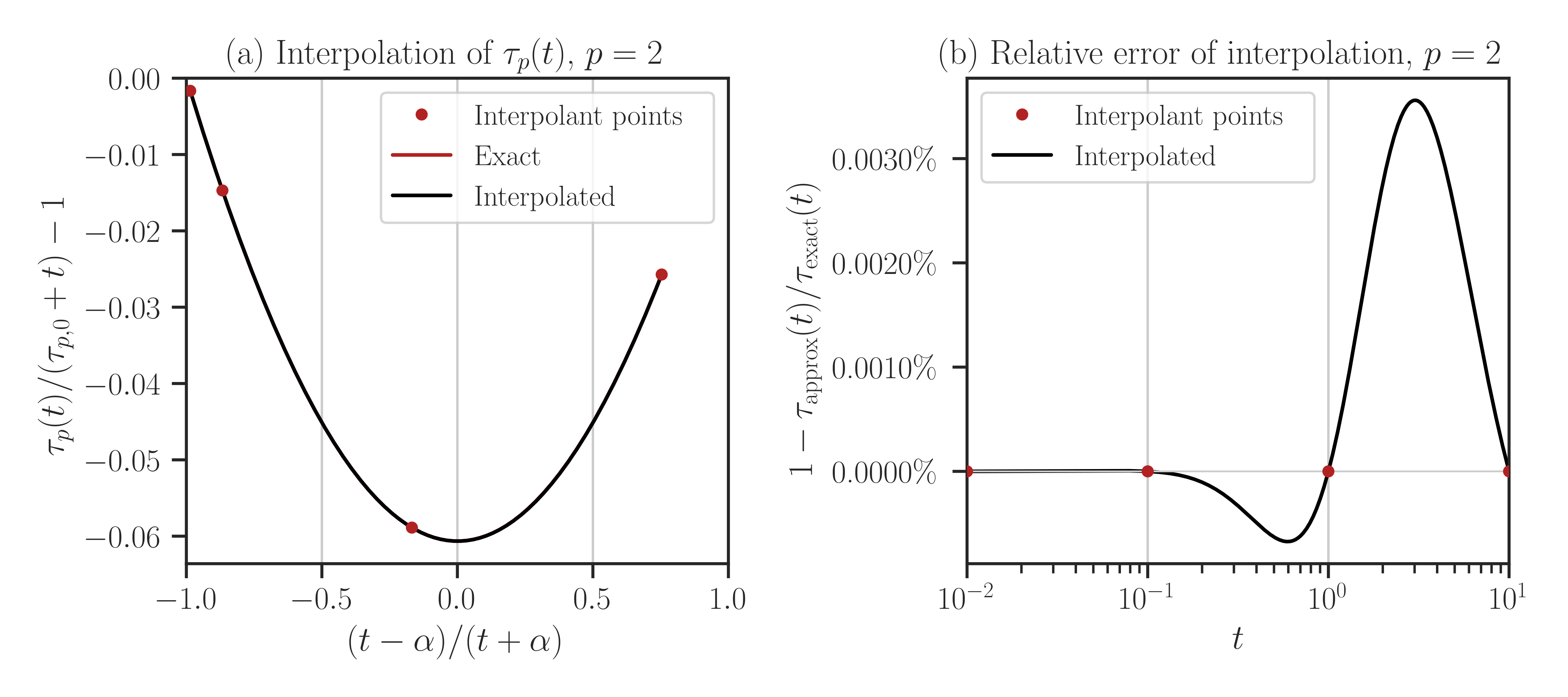
From the error plot in the above, it can be seen that with only four interpolation points, the error of interpolation for a wide range of \(t\) is no more than \(0.003 \%\). Also, note that the error on the interpolant points \(t_i=[10^{-2}, 10^{-1}, 1, 10]\) is zero since the interpolation scheme honors the exact function value at the interpolation points.

Attributes:

kindstr: Method of interpolation. For this class, kind is crf.
verbosebool: Verbosity of the computation process
nint: Size of the matrix
qint: Number of interpolant points.
pfloat: Order of Schatten \(p\)-norm

Methods

__call__	See `imate.InterpolateSchatten.__call__()`.
eval	See `imate.InterpolateSchatten.eval()`.
interpolate	See `imate.InterpolateSchatten.interpolate()`.
get_scale	See `imate.InterpolateSchatten.get_scale()`.
bound	See `imate.InterpolateSchatten.bound()`.
upper_bound	See `imate.InterpolateSchatten.upper_bound()`.
plot	See `imate.InterpolateSchatten.plot()`.