imate.InterpolateSchatten(kind=’spl’)#
- class imate.InterpolateSchatten(A, B=None, p=0, options={}, verbose=False, ti=[], kind='spl', func_type=1)
Interpolate Schatten norm (or anti-norm) of an affine matrix function using Spline (spl) method.
See also
This page describes only the spl method. For other kinds, see
imate.InterpolateSchatten().- Parameters:
- Anumpy.ndarray, scipy.sparse matrix
Symmetric positive-definite matrix (positive-definite if p is non-positive). Matrix can be dense or sparse.
Warning
Symmetry and positive (semi-) definiteness of A will not be checked. Make sure A satisfies these conditions.
- Bnumpy.ndarray, scipy.sparse matrix, default=None
Symmetric positive-definite matrix (positive-definite if p is non-positive). Matrix can be dense or sparse. B should have the same size and type of A. If B is None (default value), it is assumed that B is the identity matrix.
Warning
Symmetry and positive (semi-) definiteness of B will not be checked. Make sure B satisfies these conditions.
- pfloat, default=2
The order \(p\) in the Schatten \(p\)-norm which can be real positive, negative or zero.
- optionsdict, default={}
At each interpolation point \(t_i\), the Schatten norm is computed using
imate.schatten()function which itself calls either ofimate.logdet()(if \(p=0\))imate.trace()(if \(p>0\))imate.traceinv()(if \(p < 0\)).
The
optionspasses a dictionary of arguments to the above functions.- verbosebool, default=False
If True, it prints some information about the computation process.
- tifloat or array_like(float), default=None
Interpolation points, which can be a single number, a list or an array of interpolation points. The interpolator honors the exact function values at the interpolant points.
- func_type: {1, 2}, default=1
Type of interpolation function model. See Notes below for details.
Notes
Schatten Norm:
In this class, the Schatten \(p\)-norm of the matrix \(\mathbf{A}\) is defined by
(1)#\[\begin{split}\Vert \mathbf{A} \Vert_p = \begin{cases} \left| \mathrm{det}(\mathbf{A}) \right|^{\frac{1}{n}}, & p=0, \\ \left| \frac{1}{n} \mathrm{trace}(\mathbf{A}^{p}) \right|^{\frac{1}{p}}, & p \neq 0, \end{cases}\end{split}\]where \(n\) is the size of the matrix. When \(p \geq 0\), the above definition is the Schatten norm, and when \(p < 0\), the above is the Schatten anti-norm.
Note
Conventionally, the Schatten norm is defined without the normalizing factor \(\frac{1}{n}\) in (1). However, this factor is justified by the continuity granted by
(2)#\[\lim_{p \to 0} \Vert \mathbf{A} \Vert_p = \Vert \mathbf{A} \Vert_0.\]See [1] (Section 2) and the examples in
imate.schatten()for details.Interpolation of Affine Matrix Function:
This class interpolates the one-parameter matrix function:
\[t \mapsto \| \mathbf{A} + t \mathbf{B} \|_p,\]where the matrices \(\mathbf{A}\) and \(\mathbf{B}\) are symmetric and positive semi-definite (positive-definite if \(p < 0\)) and \(t \in [t_{\inf}, \infty)\) is a real parameter where \(t_{\inf}\) is the minimum \(t\) such that \(\mathbf{A} + t_{\inf} \mathbf{B}\) remains positive-definite.
Method of Interpolation:
Define the function
\[\tau_p(t) = \frac{\Vert \mathbf{A} + t \mathbf{B} \Vert_p} {\Vert \mathbf{B} \Vert_p},\]and \(\tau_{p, 0} = \tau_p(0)\). Then, we approximate \(\tau_p(t)\) as follows. Transform the data \((t, \tau_p)\) to \((x, y)\) where
\[x = \frac{t - 1}{t + 1},\]Also, if
func_type=1, then \(y\) is defined by\[y = \frac{\tau_p(t)}{\tau_{p, 0} + t} - 1,\]and, if
func_type=2, then \(y\) is defined by\[y = \frac{\tau_p(t) -\tau_{p, 0}}{t} - 1.\]The spline method interpolates the data \((x, y)\) by cubic splines.
Boundary Conditions:
The following boundary conditions are added to the data \((x, y)\):
If
func_typeis 1, then the two points \((-1, 0)\) and \((1, 0)\) are imposed to the spline.If
func_typeis 2, then the point \((1, 0)\) is imposed to the spline.
Interpolation Points:
The best practice is to provide an array of interpolation points that are equally distanced on the logarithmic scale. For instance, to produce four interpolation points in the interval \([10^{-2}, 1]\):
>>> import numpy
>>> ti = numpy.logspace(-2, 1, 4)
References
[1]Ameli, S., and Shadden. S. C. (2022). Interpolating Log-Determinant and Trace of the Powers of Matrix \(\mathbf{A} + t \mathbf{B}\). Statistics and Computing 32, 108. https://doi.org/10.1007/s11222-022-10173-4.
Examples
Basic Usage:
Interpolate the Schatten 2-norm of the affine matrix function \(\mathbf{A} + t \mathbf{B}\) using
splalgorithm and the interpolating points \(t_i = [10^{-2}, 10^{-1}, 1, 10]\).>>> # Generate two sample matrices (symmetric and positive-definite) >>> from imate.sample_matrices import correlation_matrix >>> A = correlation_matrix(size=20, scale=1e-1) >>> B = correlation_matrix(size=20, scale=2e-2) >>> # Initialize interpolator object >>> from imate import InterpolateSchatten >>> ti = [1e-2, 1e-1, 1, 1e1] >>> f = InterpolateSchatten(A, B, p=2, kind='spl', ti=ti, func_type=1) >>> # Interpolate at an inquiry point t = 0.4 >>> t = 4e-1 >>> f(t) 1.7372898625858328
Alternatively, call
imate.InterpolateSchatten.interpolate()to interpolate at points t:>>> # This is the same as f(t) >>> f.interpolate(t) 1.7372898625858328
To evaluate the exact value of the Schatten norm at point t without interpolation, call
imate.InterpolateSchatten.eval()function:>>> # This evaluates the function value at t exactly (no interpolation) >>> f.eval(t) 1.7374809371539666
It can be seen that the relative error of interpolation compared to the exact solution in the above is \(0.01 \%\) using only four interpolation points \(t_i\), which is a remarkable result.
Warning
Calling
imate.InterpolateSchatten.eval()may take a longer time to compute as it computes the function exactly. Particularly, if t is a large array, it may take a very long time to return the exact values.Passing Options:
The above examples, the internal computation is passed to
imate.trace()function since \(p=2\) is positive. You can pass arguments to the latter function usingoptionsargument. To do so, create a dictionary with the keys as the name of the argument. For instance, to use imate.trace(method=’slq’) method withmin_num_samples=20andmax_num_samples=100, create the following dictionary:>>> # Specify arguments as a dictionary >>> options = { ... 'method': 'slq', ... 'min_num_samples': 20, ... 'max_num_samples': 100 ... } >>> # Pass the options to the interpolator >>> f = InterpolateSchatten(A, B, p=2, options=options, kind='spl', ... ti=ti) >>> f(t) 1.7076411989963456
You may get a different result than the above as the slq method is a randomized method.
Interpolate on Range of Points:
Once the interpolation object
fin the above example is instantiated, callingimate.InterpolateSchatten.interpolate()on a list of inquiry points t has almost no computational cost. The next example inquires interpolation on 1000 points t:Interpolate an array of inquiry points
t_array:>>> # Create an interpolator object again >>> ti = 1e-1 >>> f = InterpolateSchatten(A, B, kind='spl', ti=ti) >>> # Interpolate at an array of points >>> import numpy >>> t_array = numpy.logspace(-2, 1, 1000) >>> norm_array = f.interpolate(t_array)
Plotting Interpolation and Compare with Exact Solution:
To plot the interpolation results, call
imate.InterpolateSchatten.plot()function. To compare with the true values (without interpolation), passcompare=Trueto the above function.Warning
By setting
compareto True, every point in the array t is evaluated both using interpolation and with the exact method (no interpolation). If the size of t is large, this may take a very long run time.>>> f.plot(t_array, normalize=True, compare=True)
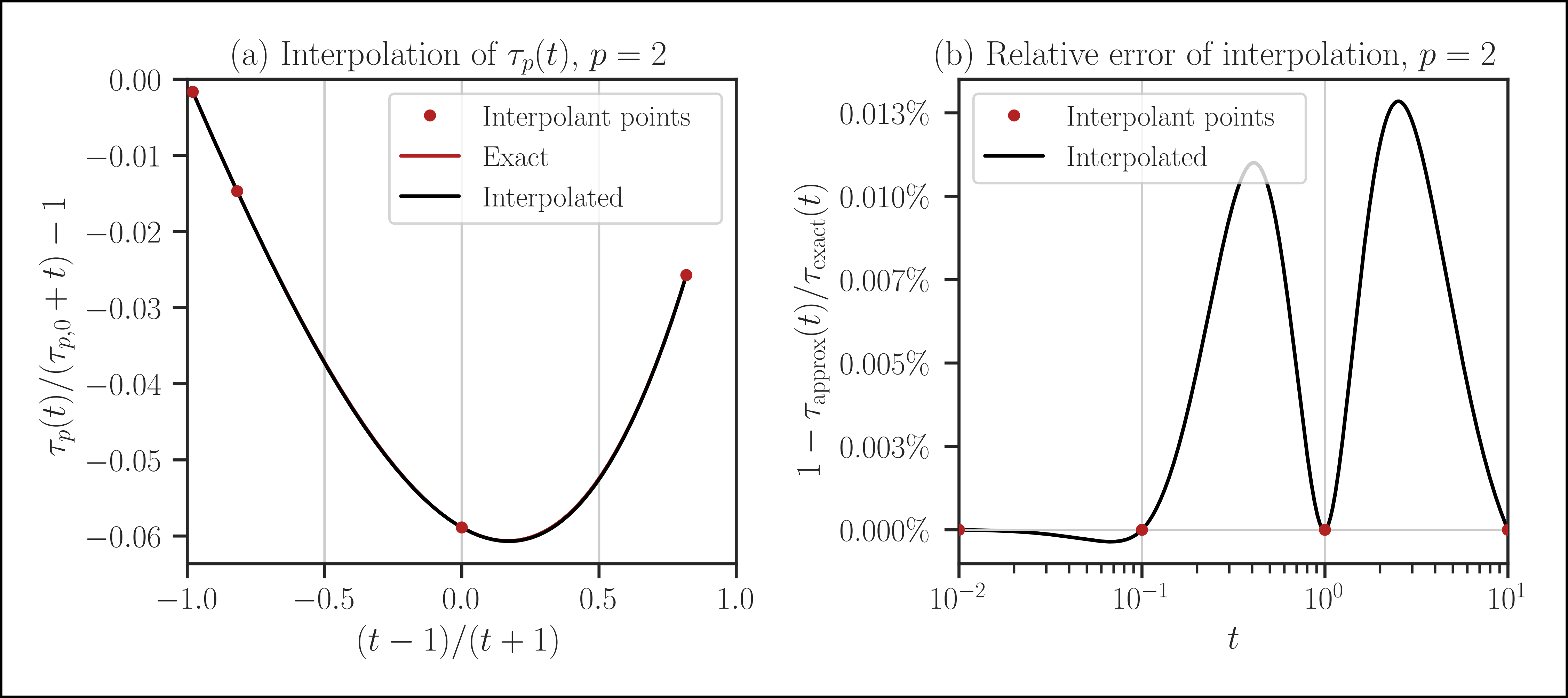
From the error plot in the above, it can be seen that with only four interpolation points, the error of interpolation for a wide range of \(t\) is no more than \(0.0013 \%\). Also, note that the error on the interpolant points \(t_i=[10^{-2}, 10^{-1}, 1, 10]\) is zero since the interpolation scheme honors the exact function value at the interpolation points.
- Attributes:
- kindstr
Method of interpolation. For this class,
kindisspl.- verbosebool
Verbosity of the computation process
- nint
Size of the matrix
- qint
Number of interpolant points.
- pfloat
Order of Schatten \(p\)-norm
Methods
__call__
eval
interpolate
bound
upper_bound
plot