imate.InterpolateSchatten#
- class imate.InterpolateSchatten(A, B=None, p=2, options={}, verbose=False, kind='imbf', ti=[], **kwargs)#
Interpolate Schatten norm (or anti-norm) of an affine matrix function.
- Parameters:
- Anumpy.ndarray, scipy.sparse matrix
Symmetric positive-definite matrix (positive-definite if p is non-positive). Matrix can be dense or sparse.
Warning
Symmetry and positive (semi-) definiteness of A will not be checked. Make sure A satisfies these conditions.
- Bnumpy.ndarray, scipy.sparse matrix, default=None
Symmetric positive-definite matrix (positive-definite if p is non-positive). Matrix can be dense or sparse. B should have the same size and type of A. If B is None (default value), it is assumed that B is the identity matrix.
Warning
Symmetry and positive (semi-) definiteness of B will not be checked. Make sure B satisfies these conditions.
- pfloat, default=2
The order \(p\) in the Schatten \(p\)-norm which can be real positive, negative or zero.
- optionsdict, default={}
At each interpolation point \(t_i\), the Schatten norm is computed using
imate.schatten()function which itself calls either ofimate.logdet()(if \(p=0\))imate.trace()(if \(p>0\))imate.traceinv()(if \(p < 0\)).
The
optionspasses a dictionary of arguments to the above functions.- verbosebool, default=False
If True, it prints some information about the computation process.
- kind{‘ext’, ‘eig’, ‘mbf’, ‘imbf’, ‘rbf’, ‘crf’, ‘spl’, ‘rpf’}, default: ‘imbf’
The algorithm of interpolation. See documentation for each specific algorithm:
- tifloat or array_like(float), default=None
Interpolation points, which can be a single point, a list, or an array of points. The interpolator honors the exact function values at the interpolant points. If an empty list is given, i.e.,
[], depending on the algorithm, a default list of interpolant points is used. Also, the size of the array of ti depends on the algorithm as follows. Ifkindis:extoreig, the notiis required.mbf, then a single pointtimay be specified.imbf,spl, orrbf, then a list oftiwith arbitrary size may be specified.crforrpf, then a list oftipoints with even size may be specified.
- kwargs**kwargs
Additional arguments to pass to each specific algorithm. See documentation for each
kindin the above.
Notes
Schatten Norm:
In this class, the Schatten \(p\)-norm of the matrix \(\mathbf{A}\) is defined by
(1)#\[\begin{split}\Vert \mathbf{A} \Vert_p = \begin{cases} \left| \mathrm{det}(\mathbf{A}) \right|^{\frac{1}{n}}, & p=0, \\ \left| \frac{1}{n} \mathrm{trace}(\mathbf{A}^{p}) \right|^{\frac{1}{p}}, & p \neq 0, \end{cases}\end{split}\]where \(n\) is the size of the matrix. When \(p \geq 0\), the above definition is the Schatten norm, and when \(p < 0\), the above is the Schatten anti-norm.
Note
Conventionally, the Schatten norm is defined without the normalizing factor \(\frac{1}{n}\) in (1). However, this factor is justified by the continuity granted by
(2)#\[\lim_{p \to 0} \Vert \mathbf{A} \Vert_p = \Vert \mathbf{A} \Vert_0.\]See [1] (Section 2) and the examples in
imate.schatten()for details.Interpolation of Affine Matrix Function:
This class interpolates the Schatten norm (or anti-norm) of the one-parameter matrix function:
\[\tau_p: t \mapsto \| \mathbf{A} + t \mathbf{B} \|_p,\]where the matrices \(\mathbf{A}\) and \(\mathbf{B}\) are symmetric and positive semi-definite (positive-definite if \(p < 0\)) and \(t \in [t_{\inf}, \infty)\) is a real parameter where \(t_{\inf}\) is the minimum \(t\) such that \(\mathbf{A} + t_{\inf} \mathbf{B}\) remains positive-definite.
The interpolator is initialized by providing \(q\) interpolant points \(t_i\), \(i = 1, \dots, q\), which are often given in a logarithmically spaced interval \(t_i \in [t_1, t_p]\). The interpolator can interpolate the above function at arbitrary inquiry points \(t \in [t_1, t_p]\) using various methods.
References
[1]Ameli, S., and Shadden. S. C. (2022). Interpolating Log-Determinant and Trace of the Powers of Matrix \(\mathbf{A} + t \mathbf{B}\). Statistics and Computing 32, 108. https://doi.org/10.1007/s11222-022-10173-4.
Examples
Basic Usage:
Interpolate the Schatten 2-norm of the affine matrix function \(\mathbf{A} + t \mathbf{B}\) using
imbfalgorithm and the interpolating points \(t_i = [10^{-2}, 10^{-1}, 1, 10]\).>>> # Generate two sample matrices (symmetric and positive-definite) >>> from imate.sample_matrices import correlation_matrix >>> A = correlation_matrix(size=20, scale=1e-1) >>> B = correlation_matrix(size=20, scale=2e-2) >>> # Initialize interpolator object >>> from imate import InterpolateSchatten >>> ti = [1e-2, 1e-1, 1, 1e1] >>> f = InterpolateSchatten(A, B, p=2, kind='imbf', ti=ti) >>> # Interpolate at an inquiry point t = 0.4 >>> t = 4e-1 >>> f(t) 1.7328745175033962
Alternatively, call
imate.InterpolateSchatten.interpolate()to interpolate at points t:>>> # This is the same as f(t) >>> f.interpolate(t) 1.7328745175033962
To evaluate the exact value of the Schatten norm at point t without interpolation, call
imate.InterpolateSchatten.eval()function:>>> # This evaluates the function value at t exactly (no interpolation) >>> f.eval(t) 1.7374809371539666
It can be seen that the relative error of interpolation compared to the exact solution in the above is \(0.26 \%\) using only four interpolation points \(t_i\), which is a remarkable result.
Warning
Calling
imate.InterpolateSchatten.eval()may take a longer time to compute as it computes the function exactly. Particularly, if t is a large array, it may take a very long time to return the exact values.Arguments Specific to Algorithms:
In the above example, the
imbfalgorithm is used. See more arguments of this algorithm at imate.InterpolateSchatten(kind=’imbf’). In the next example, we passbasis_func_typespecific to this algorithm:>>> # Passing kwatgs specific to imbf algorithm >>> f = InterpolateSchatten(A, B, p=2, kind='imbf', ti=ti, ... basis_func_type='ortho2') >>> f(t) 1.7328745175033962
You may choose other algorithms using
kindargument. For instance, the next example uses the Chebyshev rational functions with an additional argumentfunc_typespecific to this method. See more details at imate.InterpolateSchatten(kind=’crf’).>>> # Generate two sample matrices (symmetric and positive-definite) >>> f = InterpolateSchatten(A, B, p=2, kind='crf', ti=ti, ... func_type=1) >>> f(t) 1.737489512386539
Passing Options:
The above examples, the internal computation is passed to
imate.trace()function since \(p=2\) is positive. You can pass arguments to the latter function usingoptionsargument. To do so, create a dictionary with the keys as the name of the argument. For instance, to use imate.trace(method=’slq’) method withmin_num_samples=20andmax_num_samples=100, create the following dictionary:>>> # Specify arguments as a dictionary >>> options = { ... 'method': 'slq', ... 'min_num_samples': 20, ... 'max_num_samples': 100 ... } >>> # Pass the options to the interpolator >>> f = InterpolateSchatten(A, B, p=2, options=options, kind='imbf', ... ti=ti) >>> f(t) 1.7291144488066212
You may get a different result than the above as the slq method is a randomized method.
Interpolate on Range of Points:
Once the interpolation object
fin the above example is instantiated, callingimate.InterpolateSchatten.interpolate()on a list of inquiry points t has almost no computational cost. The next example inquires interpolation on 1000 points t:Interpolate an array of inquiry points
t_array:>>> # Create an interpolator object again >>> ti = [1e-2, 1e-1, 1, 1e1] >>> f = InterpolateSchatten(A, B, ti=ti) >>> # Interpolate at an array of points >>> import numpy >>> t_array = numpy.logspace(-2, 1, 1000) >>> norm_array = f.interpolate(t_array)
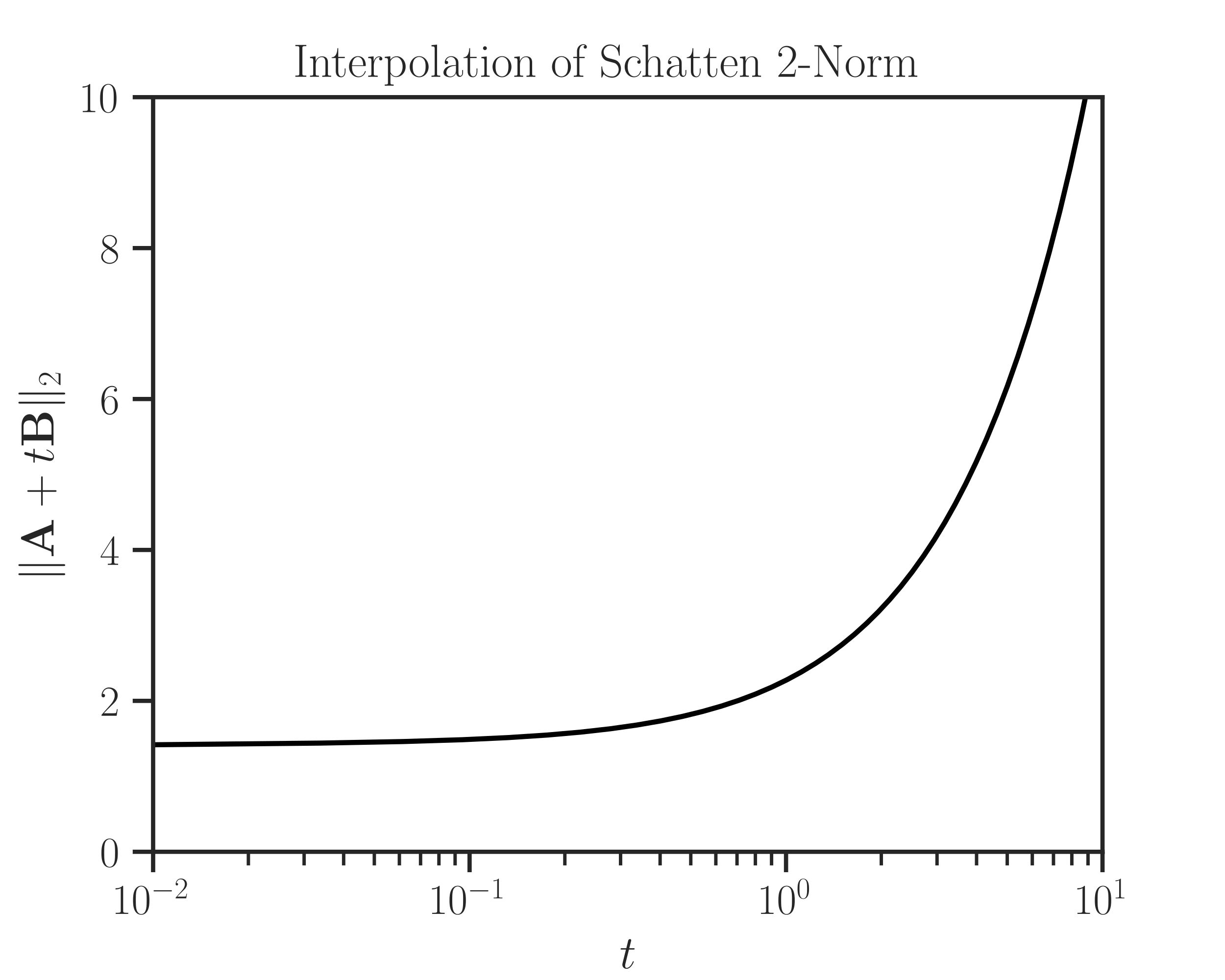
One may plot the above interpolated results as follows:
>>> import matplotlib.pyplot as plt

>>> # Plot settings (optional)
>>> from imate._utilities import set_theme
>>> set_theme(font_scale=1.15)

>>> plt.semilogx(t_array, norm_array, color='black')
>>> plt.xlim([t_array[0], t_array[-1]])
>>> plt.ylim([0, 10])
>>> plt.xlabel('$t$')
>>> plt.ylabel('$\Vert \mathbf{A} + t \mathbf{B} \Vert_{2}$')
>>> plt.title('Interpolation of Schatten 2-Norm')
>>> plt.show()
Plotting Interpolation and Compare with Exact Solution:
A more convenient way to plot the interpolation result is to call
imate.InterpolateSchatten.plot()function.>>> f.plot(t_array)
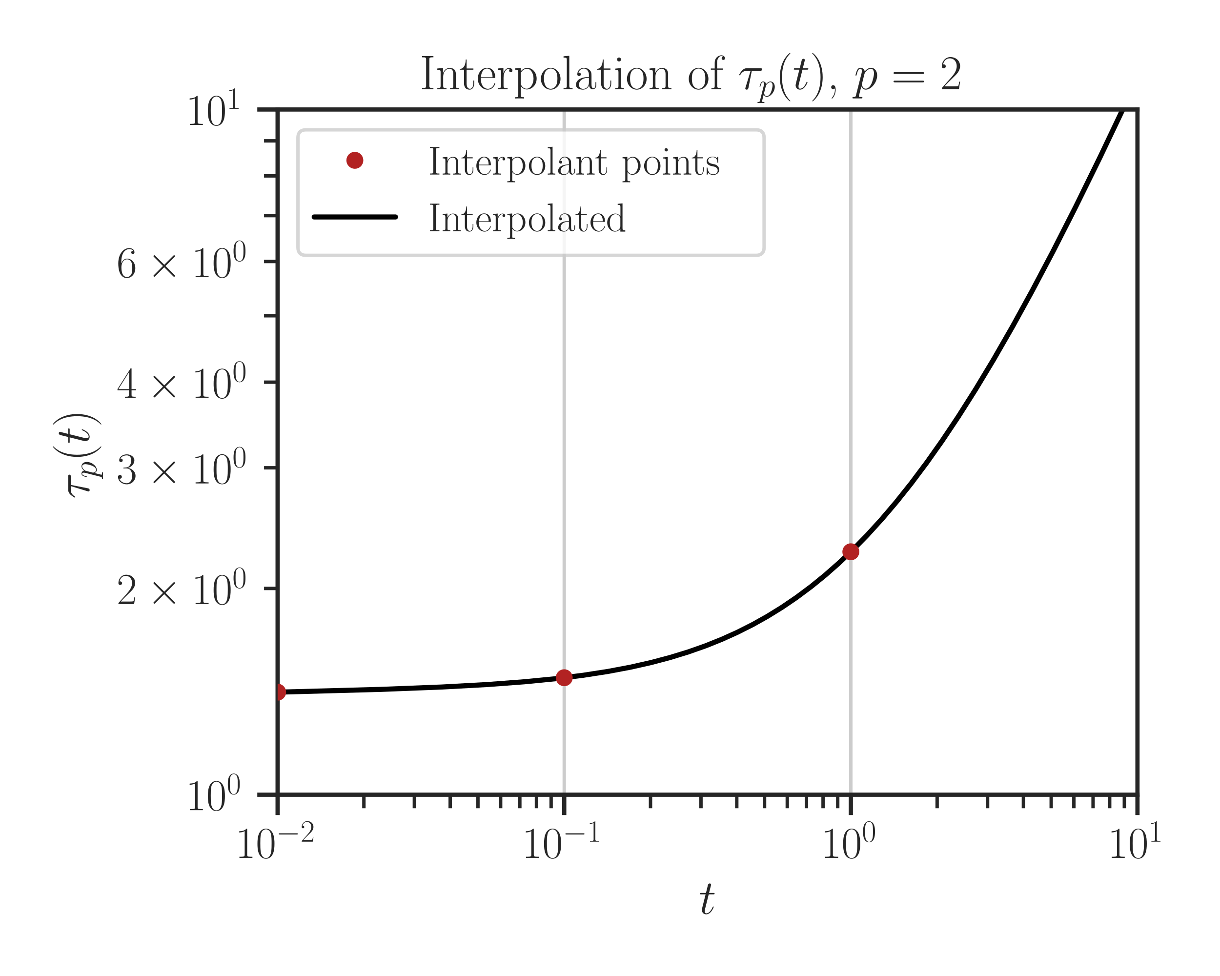
In the above, \(\tau_p = \Vert \mathbf{A} + t \mathbf{B} \Vert_p\). If you set
normalizeto True, it plots the normalized function\[\frac{\Vert \mathbf{A} + t \mathbf{B} \Vert_{p}}{ \Vert \mathbf{B} \Vert_p}.\]To compare with the true values (without interpolation), pass
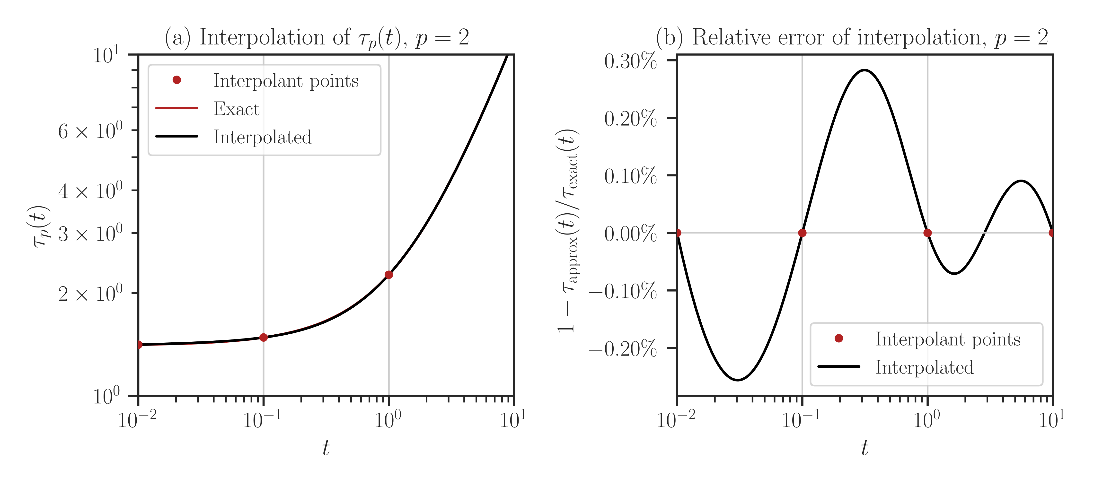
compare=Trueto the above function.Warning
By setting
compareto True, every point in the array t is evaluated both using interpolation and with the exact method (no interpolation). If the size of t is large, this may take a very long run time.>>> f.plot(t_array, normalize=True, compare=True)
- Attributes:
- kindstr
Method of interpolation
- verbosebool
Verbosity of the computation process
- nint
Size of the matrix
- qint
Number of interpolant points
- pfloat
Order of Schatten \(p\)-norm
Methods
__call__(t)Interpolate at the input point t.
eval(t)Evaluate the exact value of the function at the input point t without interpolation.
interpolate(t)Interpolate at the input point t.
Returns the scale parameter of the interpolator.
bound(t)Bound of the interpolation function.
upper_bound(t)Upper bound of the interpolation function.
plot(t[, normalize, compare, filename, verbose])Plot the interpolation results.