glearn.priors.Gamma

class glearn.priors.Gamma(shape=1.0, rate=1.0)

Gamma distribution.

Note

For the methods of this class, see the base class glearn.priors.Prior.

Parameters:

shapefloat or array_like[float], default=1.0

The shape parameter \(\alpha\) of Gamma distribution. If an array \(\boldsymbol{\alpha} = (\alpha_1, \dots, \alpha_p)\) is given, the prior is assumed to be \(p\) independent Gamma distributions each with shape \(\alpha_i\).

ratefloat or array_like[float], default=1.0

The rate \(\beta\) of Gamma distribution. If an array \(\boldsymbol{\beta} = (\beta_1, \dots, \beta_p)\) is given, the prior is assumed to be \(p\) independent Gamma distributions each with rate \(\beta_i\).

See also

glearn.priors.Prior

Notes

Single Hyperparameter:

The Gamma distribution with shape parameter \(\alpha > 0\) and rate parameter \(\beta > 0\) is defined by the probability density function

\[p(\theta \vert \alpha, \beta) = \frac{\theta^{\alpha-1} e^{-\beta \theta} \beta^{\alpha}}{\Gamma(\alpha)},\]

where \(\Gamma\) is the Gamma function.

Multiple Hyperparameters:

If an array of the hyperparameters are given, namely \(\boldsymbol{\theta} = (\theta_1, \dots, \theta_p)\), then the prior is the product of independent priors

\[p(\boldsymbol{\theta}) = p(\theta_1) \dots p(\theta_p).\]

In this case, if the input arguments shape and rate are given as the arrays \(\boldsymbol{\alpha} = (\alpha_1, \dots, \alpha_p)\) and \(\boldsymbol{\beta} = (\beta_1, \dots, \beta_p)\), each prior \(p(\theta_i)\) is defined as the Gamma distribution with shape parameter \(\alpha_i\) and rate parameter \(\beta_i\). In contrary, if shape and rate are given as the scalars \(\alpha\) and \(\beta\), then all priors \(p(\theta_i)\) are defined as the Gamma distribution with shape parameter \(\alpha\) and rate parameter \(\beta\).

Examples

Create Prior Objects:

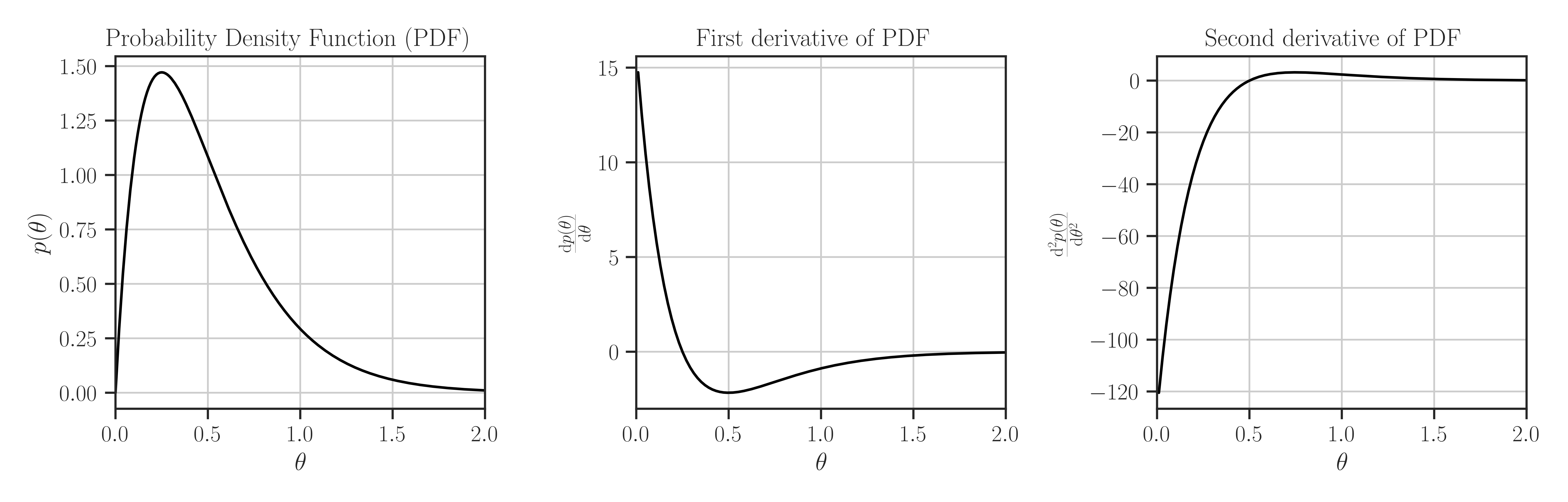
Create the Gamma distribution with the shape parameter \(\alpha=2\) and rate parameter \(\beta=4\).

>>> from glearn import priors
>>> prior = priors.Gamma(2, 4)

>>> # Evaluate PDF function at multiple locations
>>> t = [0, 0.5, 1]
>>> prior.pdf(t)
array([0.        , 1.08268227, 0.29305022])

>>> # Evaluate the Jacobian of the PDF
>>> prior.pdf_jacobian(t)
array([        nan, -2.16536453, -0.87915067])

>>> # Evaluate the Hessian of the PDF
>>> prior.pdf_hessian(t)
array([[       nan, 0.        , 0.        ],
       [0.        , 0.        , 0.        ],
       [0.        , 0.        , 2.34440178]])

>>> # Evaluate the log-PDF
>>> prior.log_pdf(t)
-44.87746683446311

>>> # Evaluate the Jacobian of the log-PDF
>>> prior.log_pdf_jacobian(t)
array([ -6.90775528, -26.82306851, -89.80081863])

>>> # Evaluate the Hessian of the log-PDF
>>> prior.log_pdf_hessian(t)
array([[ -21.20759244,    0.        ,    0.        ],
       [   0.        ,  -67.06429581,    0.        ],
       [   0.        ,    0.        , -212.07592442]])

>>> # Plot the distribution and its first and second derivative
>>> prior.plot()

Where to Use the Prior object:

Define a covariance model (see glearn.Covariance) where its scale parameter is a prior function.

>>> # Generate a set of sample points
>>> from glearn.sample_data import generate_points
>>> points = generate_points(num_points=50)

>>> # Create covariance object of the points with the above kernel
>>> from glearn import covariance
>>> cov = glearn.Covariance(points, kernel=kernel, scale=prior)

Attributes:

shapefloat or array_like[float], default=0

Shape parameter \(\alpha\) of the distribution

ratefloat or array_like[float], default=0

Rate parameter \(\beta\) of the distribution

Methods

suggest_hyperparam([positive])	Find an initial guess for the hyperparameters based on the peaks of the prior distribution.
pdf(x)	Probability density function of the prior distribution.
pdf_jacobian(x)	Jacobian of the probability density function of the prior distribution.
pdf_hessian(x)	Hessian of the probability density function of the prior distribution.