glearn.priors.BetaPrime

class glearn.priors.BetaPrime(alpha=1.0, beta=1.0)

Beta Prime distribution.

Note

For the methods of this class, see the base class glearn.priors.Prior.

Parameters:

shapefloat or array_like[float], default=1.0

The shape parameter \(\alpha\) of beta prime distribution. If an array \(\boldsymbol{\alpha} = (\alpha_1, \dots, \alpha_p)\) is given, the prior is assumed to be \(p\) independent beta prime distributions each with shape \(\alpha_i\).

ratefloat or array_like[float], default=1.0

The rate \(\beta\) of beta prime distribution. If an array \(\boldsymbol{\beta} = (\beta_1, \dots, \beta_p)\) is given, the prior is assumed to be \(p\) independent beta prime distributions each with rate \(\beta_i\).

See also

glearn.priors.Prior

Notes

Single Hyperparameter:

The beta prime distribution with shape parameter \(\alpha > 0\) and rate parameter \(\beta > 0\) is defined by the probability density function

\[p(\theta \vert \alpha, \beta) = \frac{\theta^{\alpha-1} (1+\theta)^{-(\alpha+\beta)}} {B(\alpha, \beta)},\]

where \(B\) is the Beta function.

Multiple Hyperparameters:

If an array of the hyperparameters are given, namely \(\boldsymbol{\theta} = (\theta_1, \dots, \theta_p)\), then the prior is the product of independent priors

\[p(\boldsymbol{\theta}) = p(\theta_1) \dots p(\theta_p).\]

In this case, if the input arguments shape and rate are given as the arrays \(\boldsymbol{\alpha} = (\alpha_1, \dots, \alpha_p)\) and \(\boldsymbol{\beta} = (\beta_1, \dots, \beta_p)\), each prior \(p(\theta_i)\) is defined as the beta prime distribution with shape parameter \(\alpha_i\) and rate parameter \(\beta_i\). In contrary, if shape and rate are given as the scalars \(\alpha\) and \(\beta\), then all priors \(p(\theta_i)\) are defined as the beta prime distribution with shape parameter \(\alpha`and rate parameter :math:\)beta`.

Examples

Create Prior Objects:

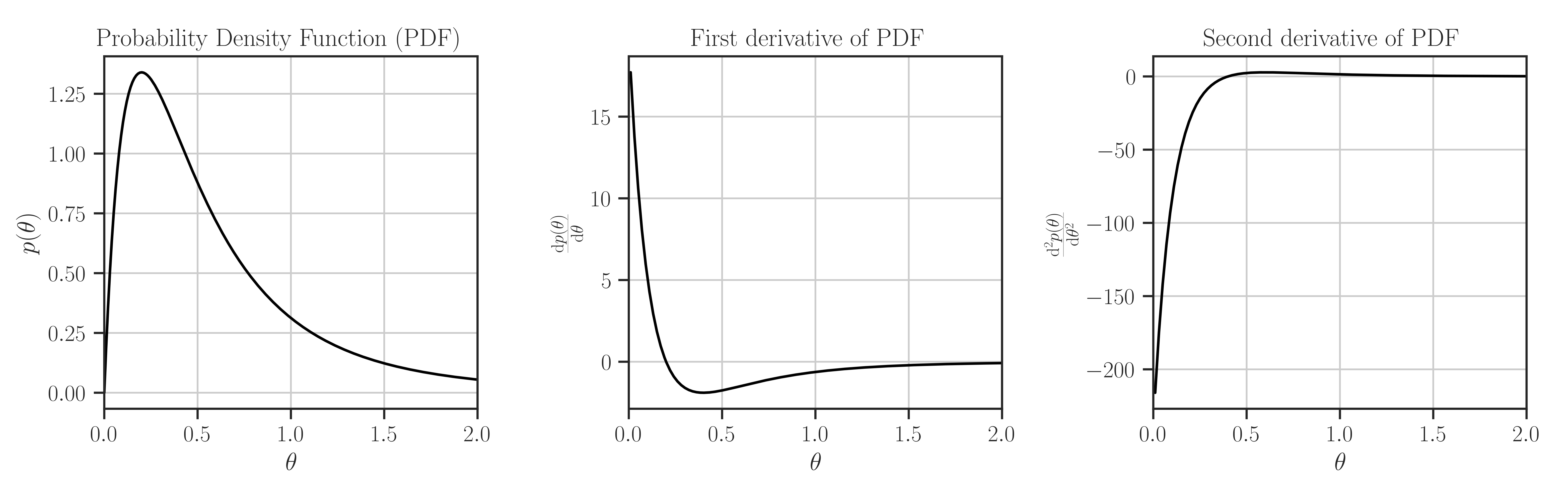
Create the beta prime distribution with the shape parameter \(\alpha=2\) and rate parameter \(\beta=4\).

>>> from glearn import priors
>>> prior = priors.BetaPrime(2, 4)

>>> # Evaluate PDF function at multiple locations
>>> t = [0, 0.5, 1]
>>> prior.pdf(t)
array([0.        , 0.87791495, 0.3125    ])

>>> # Evaluate the Jacobian of the PDF
>>> prior.pdf_jacobian(t)
array([       nan, -1.7558299, -0.625    ])

>>> # Evaluate the Hessian of the PDF
>>> prior.pdf_hessian(t)
array([[       nan, 0.        , 0.        ],
       [0.        , 2.34110654, 0.        ],
       [0.        , 0.        , 1.40625   ]])

>>> # Evaluate the log-PDF
>>> prior.log_pdf(t)
14.661554893429063

>>> # Evaluate the Jacobian of the log-PDF
>>> prior.log_pdf_jacobian(t)
array([ -4.60517019,  -8.19370659, -10.25696996])

>>> # Evaluate the Hessian of the log-PDF
>>> prior.log_pdf_hessian(t)
array([[-7.95284717,  0.        ,  0.        ],
       [ 0.        , -5.80658157,  0.        ],
       [ 0.        ,  0.        , -2.62904039]])

>>> # Plot the distribution and its first and second derivative
>>> prior.plot()

Where to Use the Prior object:

Define a covariance model (see glearn.Covariance) where its scale parameter is a prior function.

>>> # Generate a set of sample points
>>> from glearn.sample_data import generate_points
>>> points = generate_points(num_points=50)

>>> # Create covariance object of the points with the above kernel
>>> from glearn import covariance
>>> cov = glearn.Covariance(points, kernel=kernel, scale=prior)

Attributes:

shapefloat or array_like[float], default=0

Shape parameter \(\alpha\) of the distribution

ratefloat or array_like[float], default=0

Rate parameter \(\beta\) of the distribution

Methods

suggest_hyperparam([positive])	Find an initial guess for the hyperparameters based on the peaks of the prior distribution.
pdf(x)	Probability density function of the prior distribution.
pdf_jacobian(x)	Jacobian of the probability density function of the prior distribution.
pdf_hessian(x)	Hessian of the probability density function of the prior distribution.