glearn.priors.StudentT

class glearn.priors.StudentT(dof=1.0, half=False)

Student’s t-distribution.

Note

For the methods of this class, see the base class glearn.priors.Prior.

Parameters:

doffloat or array_like[float], default=1.0

Degrees of freedom \(\nu\) of Student’ t-distribution. If an array \(\boldsymbol{\nu} = (\nu_1, \dots, \nu_p)\) is given, the prior is assumed to be \(p\) independent Student’s t-distributions each with degrees of freedom \(\nu_i\).

halfbool, default=False

If True, the prior is the half-normal distribution.

See also

glearn.priors.Prior

Notes

Single Hyperparameter:

The Student’s t-distribution with degrees of freedom \(\nu\) is defined by the probability density function

\[p(\theta \vert \nu) = \frac{\Gamma(\nu')}{\sqrt{\nu \pi} \Gamma(\frac{\nu}{2})} z^{-\nu'}.\]

where \(\nu' = \frac{1 + \nu}{2}\), \(\Gamma\) is the Gamma function, and

\[z = 1 + \frac{\theta^2}{\nu}.\]

If half is True, the prior is the half Student’s t-distribution for \(\theta \geq 0\) is

\[p(\theta \vert \nu) = 2 \frac{\Gamma(\nu')}{\sqrt{\nu \pi} \Gamma(\frac{\nu}{2})} z^{-\nu'}.\]

Multiple Hyperparameters:

If an array of the hyperparameters are given, namely \(\boldsymbol{\theta} = (\theta_1, \dots, \theta_p)\), then the prior is the product of independent priors

\[p(\boldsymbol{\theta}) = p(\theta_1) \dots p(\theta_p).\]

In this case, if the input arguments dof is given as the array \(\boldsymbol{\nu} = (\nu_1, \dots, \nu_p)\) each prior \(p(\theta_i)\) is defined as the Student’s t-distribution with the degrees of freedom \(\nu_i\). In contrary, if dof is given by the scalar \(\nu\), then all priors \(p(\theta_i)\) are defined as the Student’st-distribution with degrees of freedom \(\nu\).

Examples

Create Prior Objects:

Create the Student’ t-distribution with the degrees of freedom \(\nu=4\).

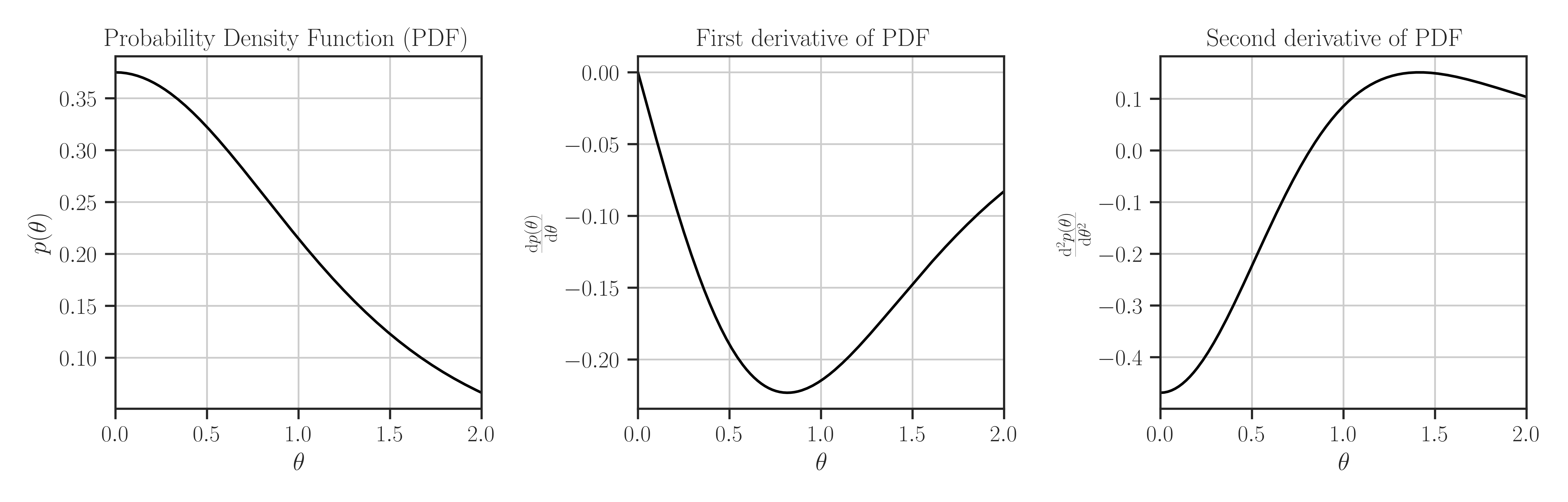
>>> from glearn import priors
>>> prior = priors.StudentT(4)

>>> # Evaluate PDF function at multiple locations
>>> t = [0, 0.5, 1]
>>> prior.pdf(t)
array([-0.        , -0.18956581, -0.21466253])

>>> # Evaluate the Jacobian of the PDF
>>> prior.pdf_jacobian(t)
array([ 0.01397716,  0.00728592, -0.        ])

>>> # Evaluate the Hessian of the PDF
>>> prior.pdf_hessian(t)
array([[-0.46875   ,  0.        ,  0.        ],
       [ 0.        , -0.22301859,  0.        ],
       [ 0.        ,  0.        ,  0.08586501]])

>>> # Evaluate the log-PDF
>>> prior.log_pdf(t)
14.777495403612827

>>> # Evaluate the Jacobian of the log-PDF
>>> prior.log_pdf_jacobian(t)
array([ -2.30258509,  -8.22351819, -11.07012064])

>>> # Evaluate the Hessian of the log-PDF
>>> prior.log_pdf_hessian(t)
array([[ -8.48303698,   0.        ,   0.        ],
       [  0.        , -10.82020023,   0.        ],
       [  0.        ,   0.        ,  -1.96076114]])

>>> # Plot the distribution and its first and second derivative
>>> prior.plot()

Where to Use the Prior object:

Define a covariance model (see glearn.Covariance) where its scale parameter is a prior function.

>>> # Generate a set of sample points
>>> from glearn.sample_data import generate_points
>>> points = generate_points(num_points=50)

>>> # Create covariance object of the points with the above kernel
>>> from glearn import covariance
>>> cov = glearn.Covariance(points, kernel=kernel, scale=prior)

Attributes:

doffloat or array_like[float], default=0

Degrees of freedom \(\nu\) of the distribution

Methods

suggest_hyperparam([positive])	Find an initial guess for the hyperparameters based on the peaks of the prior distribution.
pdf(x)	Probability density function of the prior distribution.
pdf_jacobian(x)	Jacobian of the probability density function of the prior distribution.
pdf_hessian(x)	Hessian of the probability density function of the prior distribution.