glearn.priors.Normal

class glearn.priors.Normal(mean=0.0, std=1.0, half=False)

Normal distribution.

Note

For the methods of this class, see the base class glearn.priors.Prior.

Parameters:

meanfloat or array_like[float], default=0.0

The mean \(\mu\) of normal distribution. If an array \(\boldsymbol{\mu} = (\mu_1, \dots, \mu_p)\) is given, the prior is assumed to be \(p\) independent normal distributions each with mean \(\mu_i\).

stdfloat or array_like[float], default=1.0

The standard deviation \(\sigma\) of normal distribution. If an array \(\boldsymbol{\sigma} = (\sigma_1, \dots, \sigma_p)\) is given, the prior is assumed to be \(p\) independent normal distributions each with standard deviation \(\sigma_i\).

halfbool, default=False

If True, the prior is the half-normal distribution.

See also

glearn.priors.Prior

Notes

Single Hyperparameter:

The normal distribution \(\mathcal{N}(\mu, \sigma^2)\) is defined by the probability density function

\[p(\theta \vert \mu, \sigma^2) = \frac{1}{\sigma \sqrt{2 \pi}} e^{-\frac{1}{2}z^2},\]

where

\[z = \frac{\theta - \mu}{\sigma}.\]

If half is True, the prior is the half-normal distribution for \(\theta \geq 0\) is

\[p(\theta \vert \mu, \sigma^2) = \frac{\sqrt{2}}{\sigma \sqrt{\pi}} e^{-\frac{1}{2}z^2},\]

Multiple Hyperparameters:

If an array of the hyperparameters are given, namely \(\boldsymbol{\theta} = (\theta_1, \dots, \theta_p)\), then the prior is the product of independent priors

\[p(\boldsymbol{\theta}) = p(\theta_1) \dots p(\theta_p).\]

In this case, if the input arguments mean and std are given as the arrays \(\boldsymbol{\mu} = (\mu_1, \dots, \mu_p)\) and \(\boldsymbol{\sigma} = (\sigma_1, \dots, \sigma_p)\), each prior \(p(\theta_i)\) is defined as the normal distribution \(\mathcal{N}(\mu_i, \sigma_i^2)\). In contrary, if mean and sigma are given as the scalars \(\mu\) and \(\sigma\), then all priors \(p(\theta_i)\) are defined as the normal distribution \(\mathcal{N}(\mu, \sigma^2)\).

Examples

Create Prior Objects:

Create the normal distribution \(\mathcal{N}(1, 3^2)\):

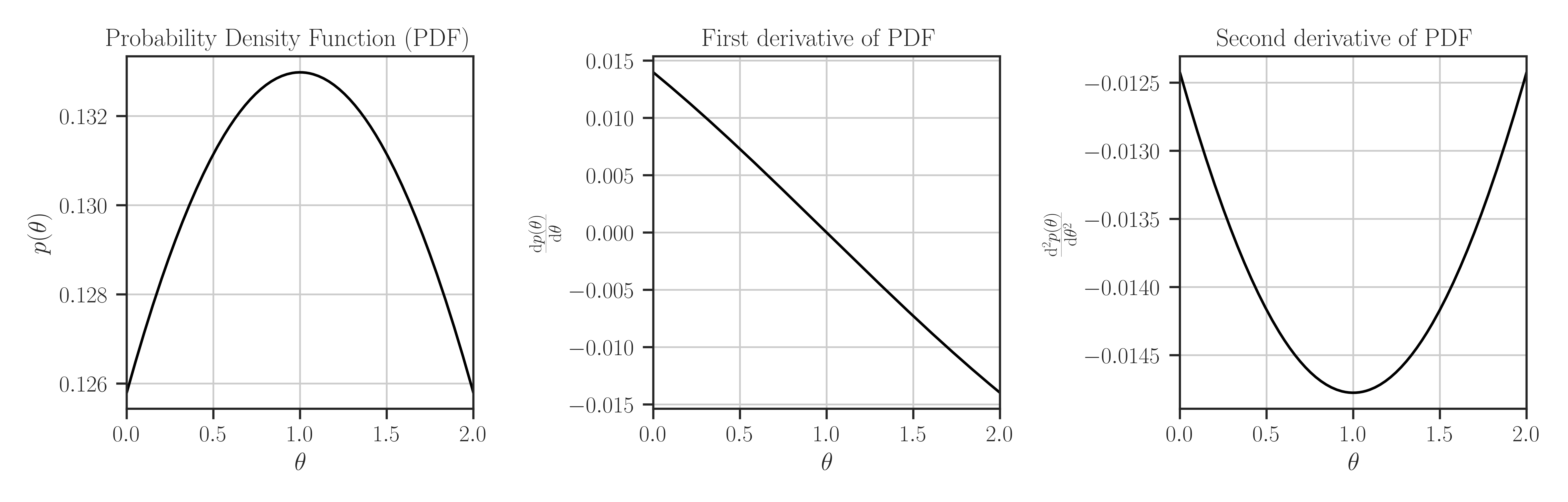
>>> from glearn import priors
>>> prior = priors.Normal(1, 3)

>>> # Evaluate PDF function at multiple locations
>>> t = [0, 0.5, 1]
>>> prior.pdf(t)
array([0.12579441, 0.13114657, 0.13298076])

>>> # Evaluate the Jacobian of the PDF
>>> prior.pdf_jacobian(t)
array([ 0.01397716,  0.00728592, -0.        ])

>>> # Evaluate the Hessian of the PDF
>>> prior.pdf_hessian(t)
array([[-0.01242414,  0.        ,  0.        ],
       [ 0.        , -0.01416707,  0.        ],
       [ 0.        ,  0.        , -0.01477564]])

>>> # Evaluate the log-PDF
>>> prior.log_pdf(t)
-10.812399392266304

>>> # Evaluate the Jacobian of the log-PDF
>>> prior.log_pdf_jacobian(t)
array([ -0.        ,  -1.74938195, -23.02585093])

>>> # Evaluate the Hessian of the log-PDF
>>> prior.log_pdf_hessian(t)
array([[  -0.58909979,    0.        ,    0.        ],
       [   0.        ,   -9.9190987 ,    0.        ],
       [   0.        ,    0.        , -111.92896011]])

>>> # Plot the distribution and its first and second derivative
>>> prior.plot()

Where to Use the Prior object:

Define a covariance model (see glearn.Covariance) where its scale parameter is a prior function.

>>> # Generate a set of sample points
>>> from glearn.sample_data import generate_points
>>> points = generate_points(num_points=50)

>>> # Create covariance object of the points with the above kernel
>>> from glearn import covariance
>>> cov = glearn.Covariance(points, kernel=kernel, scale=prior)

Attributes:

meanfloat or array_like[float], default=0

Mean of the distribution

stdfloat or array_like[float], default=0

Standard deviation of the distribution

Methods

suggest_hyperparam([positive])	Find an initial guess for the hyperparameters based on the peaks of the prior distribution.
pdf(x)	Probability density function of the prior distribution.
pdf_jacobian(x)	Jacobian of the probability density function of the prior distribution.
pdf_hessian(x)	Hessian of the probability density function of the prior distribution.