imate.InterpolateSchatten.plot#
- InterpolateSchatten.plot(t, normalize=True, compare=False, filename=None, verbose=False)#
Plot the interpolation results.
- Parameters:
- tnumpy.array
Inquiry points to be interpolated.
- normalizebool, default: False
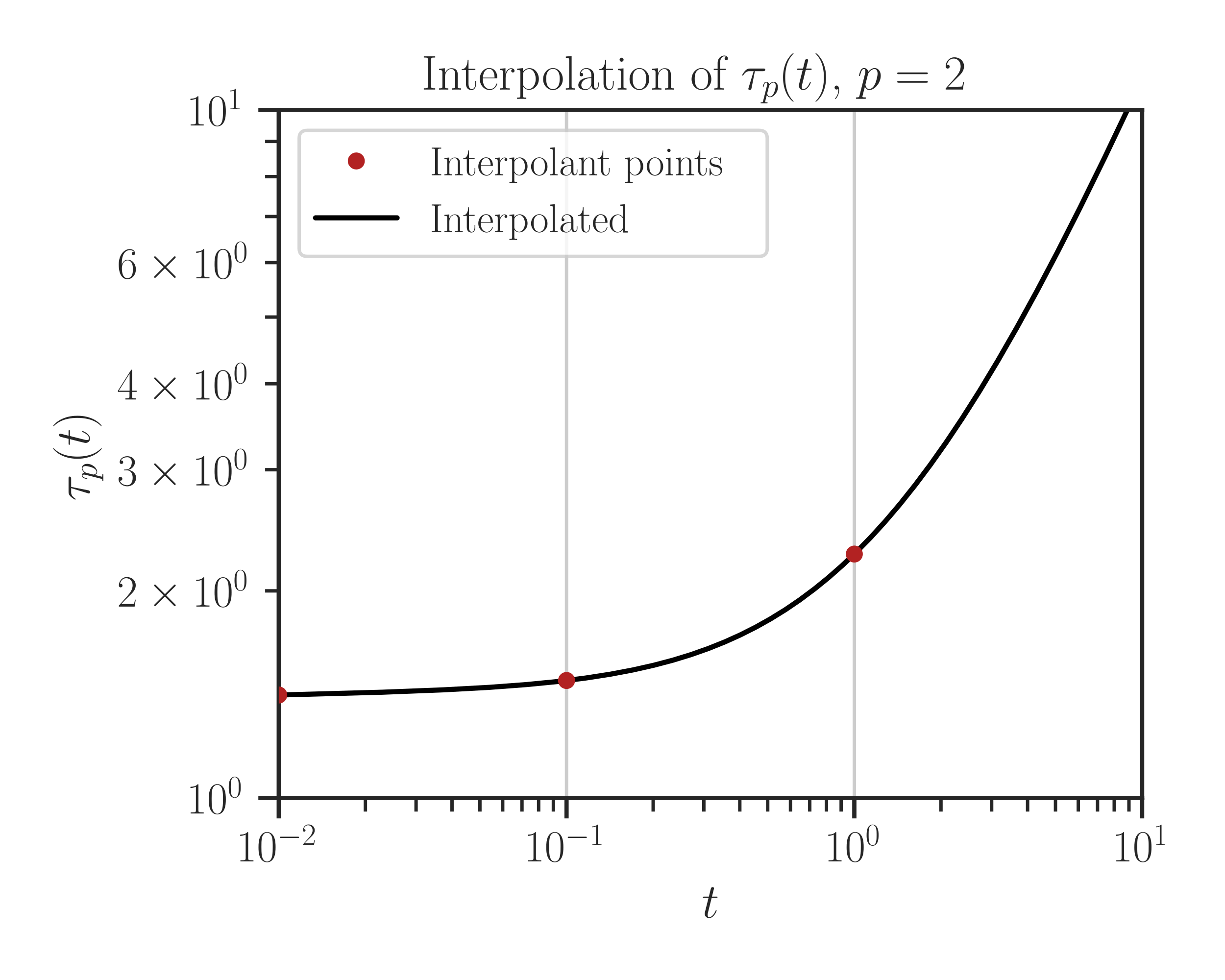
If set to False the function \(\tau_p = \Vert \mathbf{A} + t \mathbf{B} \Vert_p\) is plotted. If set to True, it plots the normalized function
\[\tau_p(t) = \frac{\Vert \mathbf{A} + t \mathbf{B} \Vert_{p}}{\Vert \mathbf{B} \Vert_p}.\]- comparebool, default=False
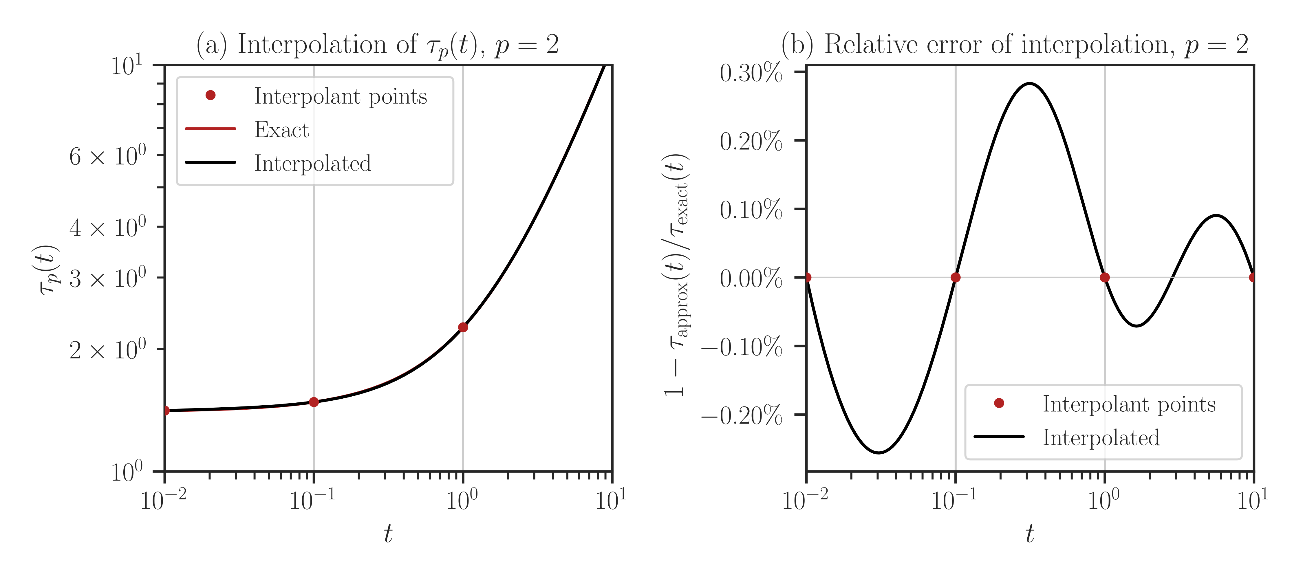
If True, it computes the exact function values (without interpolation), then compares it with the interpolated solution to estimate the relative error of interpolation.
Note
When this option is enabled, the exact solution will be computed for all inquiry points, which can take a very long time.
- filenamestr, default=False
A filename to save the file. In this case, the plot will not be shown, bit saved to a file only. If None, plot will not be saved.
- verbosebool, default=False
If True, the location os saved plot is printed.
- Raises:
- ImportError
If matplotlib is not installed.
- ValueError
If
tis not an array of size greater than one.
Notes
Plotted Function:
When
kindis either ofext,eig,mbf,imbf,rpf, orrbf, the function \(\tau_p(t)\) is plotted, which is defined as follows. Ifnormalizeis False, then\[\tau_p(t) = \Vert \mathbf{A} + t \mathbf{B} \Vert_p.\]If
normalizeis True, then\[\frac{\Vert \mathbf{A} + t \mathbf{B} \Vert_{p}}{ \Vert \mathbf{B} \Vert_p}.\]On the other hand, if
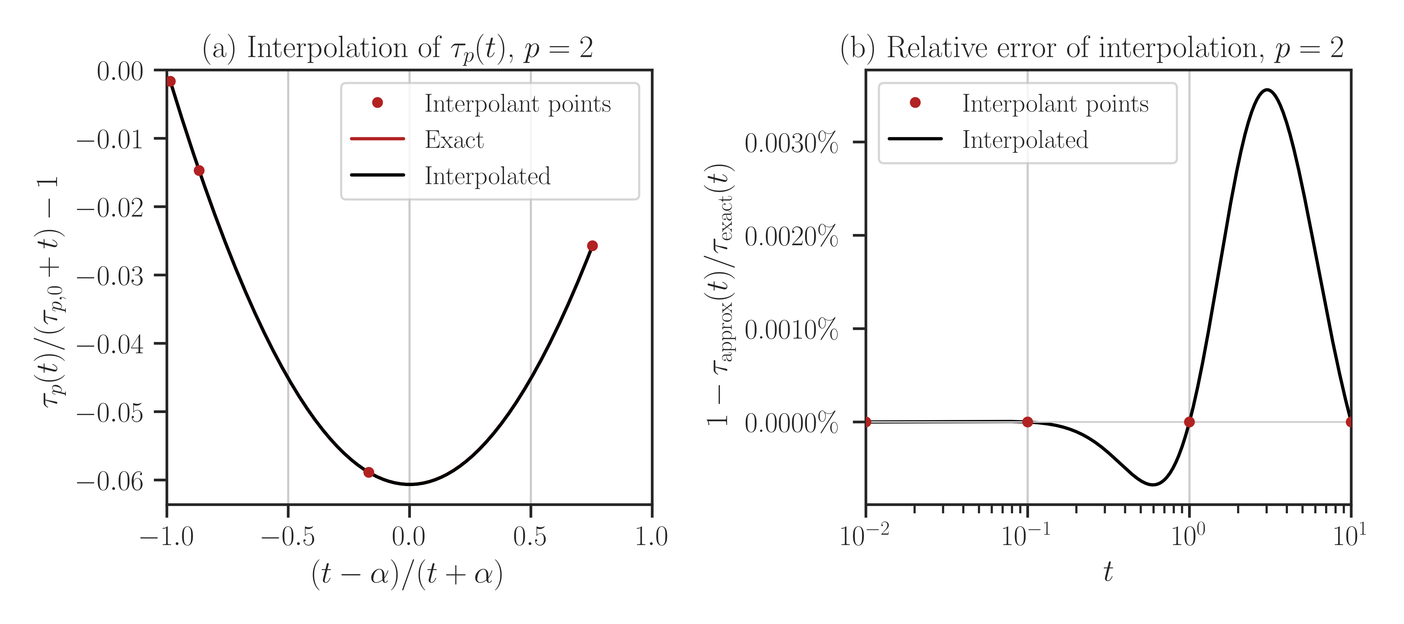
kind=crforkind=spl, the function \(y_p(x)\) is plotted, which is defined as follows:\[x = \frac{t - \alpha}{t + \alpha},\]where \(\alpha\) is the
scaleparameter in imate.InterpolateSchatten(kind=’crf’) forkind=crf. Ifkind=spl, then \(\alpha=1\). Also\[y_p = \frac{\tau_p(t)}{\tau_p(0) + t} - 1.\]
Graphical Backend:
If no graphical backend exists (such as running the code on a remote server or manually disabling the X11 backend), the plot will not be shown, rather, it will ve saved as an
svgfile in the current directory.If the executable
latexis on the path, the plot is rendered using \(\rm\LaTeX\), which then, it takes a bit longer to produce the plot.If \(\rm\LaTeX\) is not installed, it uses any available San-Serif font to render the plot.
To manually disable interactive plot display, and save the plot as
SVGinstead, add the following in the very beginning of your code before importingimate:>>> import os >>> os.environ['IMATE_NO_DISPLAY'] = 'True'
Examples
Create an interpolator object \(f\) using four interpolant points \(t_i\):
>>> # Generate sample matrices (symmetric positive-definite)
>>> from imate.sample_matrices import correlation_matrix
>>> A = correlation_matrix(size=20, scale=1e-1)
>>> B = correlation_matrix(size=20, scale=2e-2)

>>> # Initialize interpolator object
>>> from imate import InterpolateSchatten
>>> ti = [1e-2, 1e-1, 1, 1e1]
>>> f = InterpolateSchatten(A, B, ti=ti)
Define an array if inquiry point t and call
imate.InterpolateSchatten.plot()function to plot the interpolation of the function \(f(t)\):>>> import numpy >>> t_array = numpy.logspace(-2, 1, 1000) >>> f.plot(t_array)
To compare with the true values (without interpolation), pass
compare=Trueto the above function.Warning
By setting
compareto True, every point in the array t is evaluated both using interpolation and with the exact method (no interpolation). If the size of t is large, this may take a very long run time.>>> f.plot(t_array, normalize=True, compare=True)
Plotting for Chebyshev and Spline Methods:
As mentioned in the Notes in the above, if
kind=crforkind=spl, the transformed function \(y_p(x)\) is plotted as shown in the example below:>>> # Recreate interpolating object, but using crf method >>> f = InterpolateSchatten(A, B, kind='crf', ti=ti) >>> t_array = numpy.logspace(-2, 1, 1000) >>> f.plot(t_array)