glearn.GaussianProcess.plot_likelihood

GaussianProcess.plot_likelihood()

Plot the likelihood function and its derivatives with respect to the hyperparameters.

Note

The model should be pre-trained before calling this function.

Notes

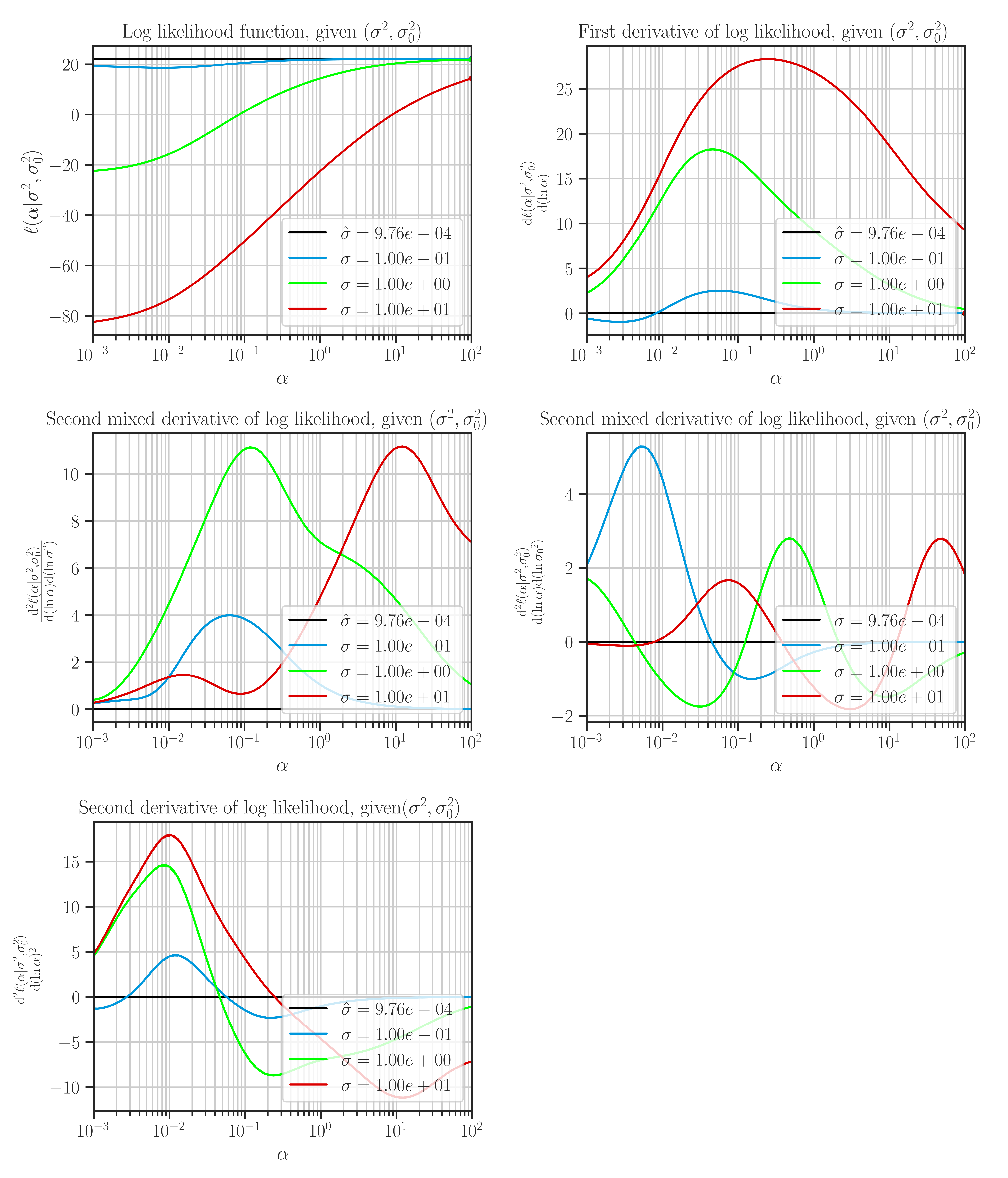
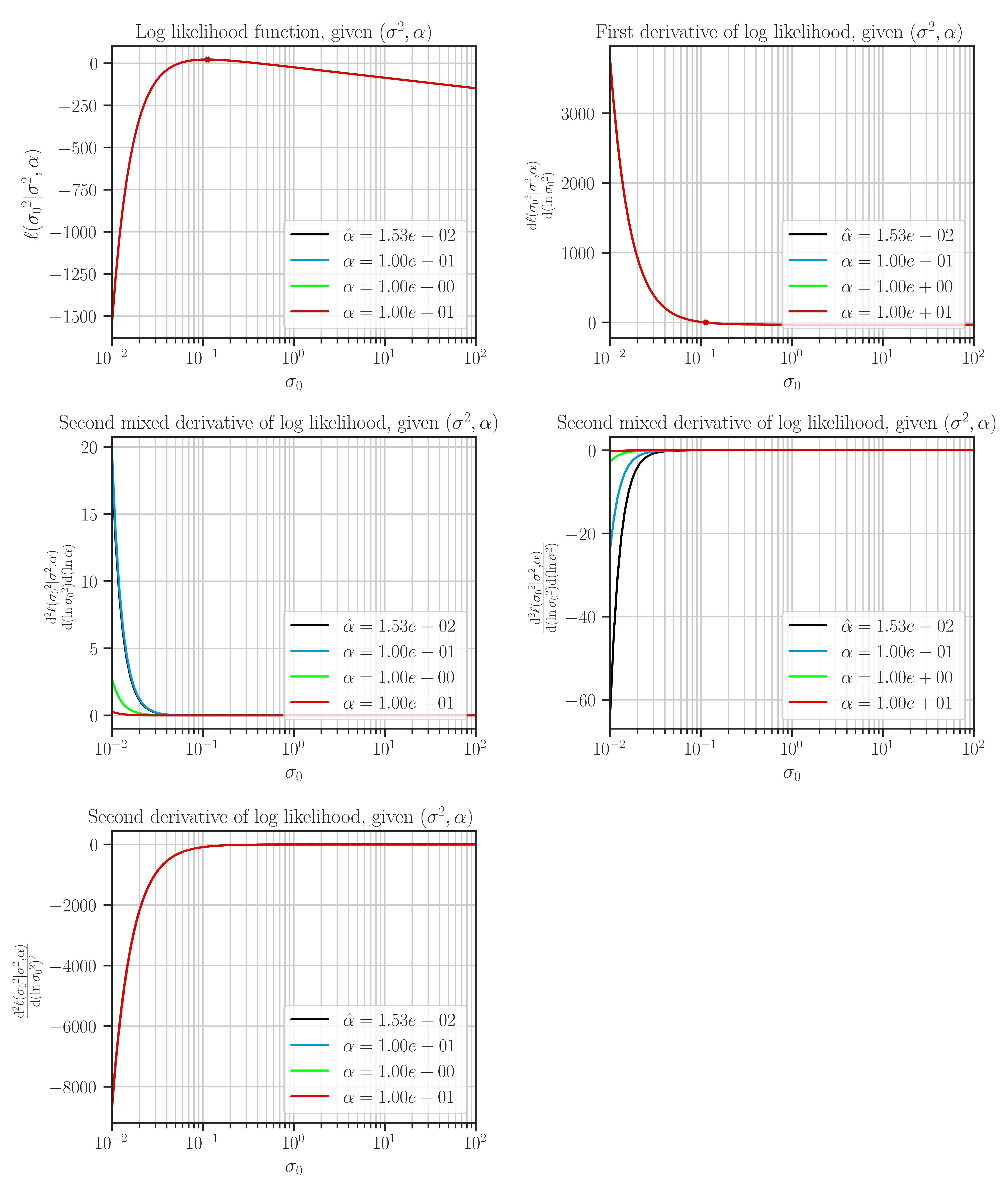
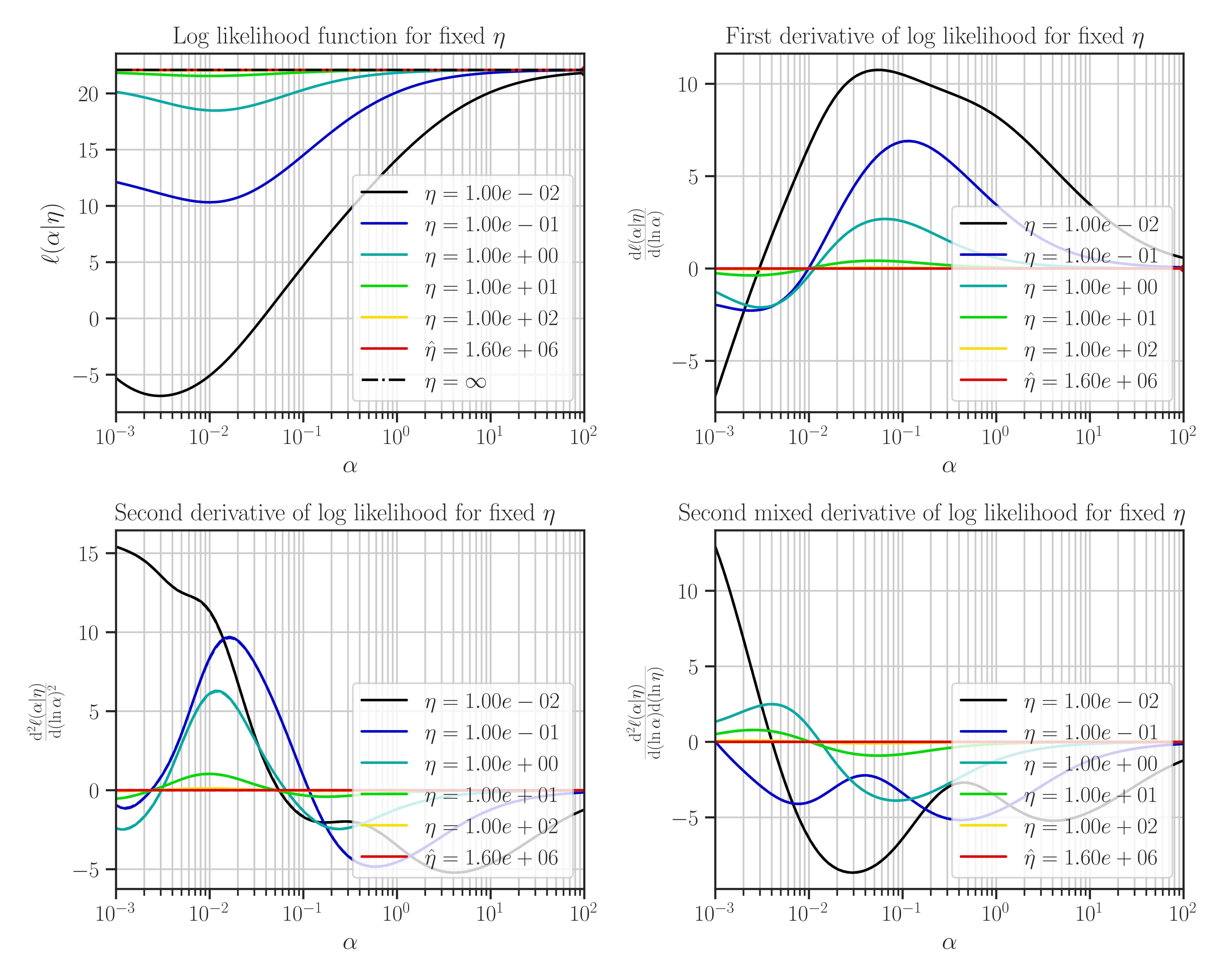
This function plots likelihood function and its first and second derivatives with respect to the hyperparameters. The type of hyperparameters depend on the profiling method which is set by profile_hyperparam.

This function is only used for testing purposes, and can only plot 1D and 2D data.

Warning

This function may take a long time, and is only used for testing purposes on small datasets.

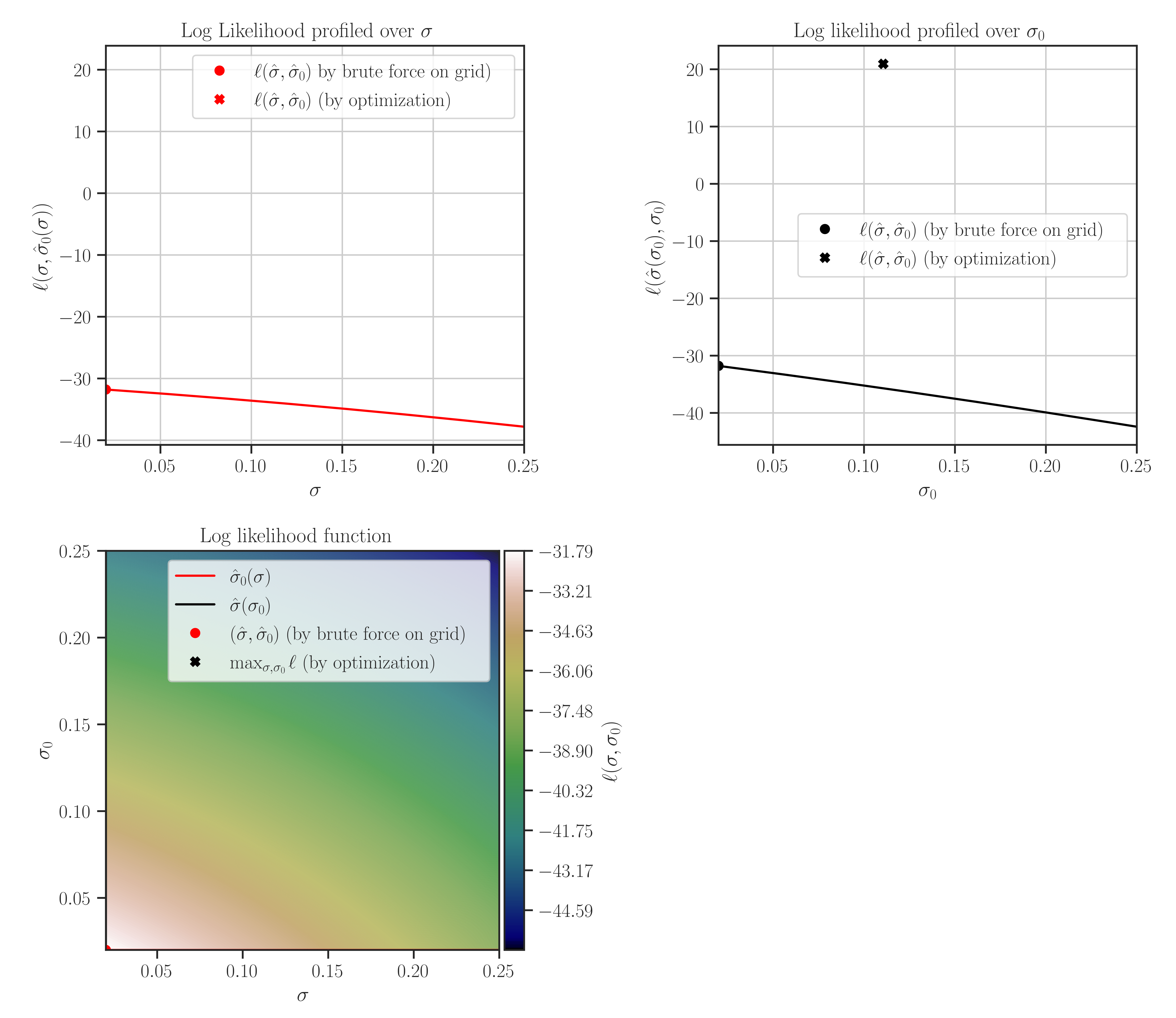
Note that the maximum points of the likelihood plots may not correspond to the optimal values of the hyperparameters. This is because the hyperparameters are found by the maximum points of the posterior function. If the prior for the scale hyperparameter is the uniform distribution, then the likelihood and the posterior functions are them same and the maxima of the likelihood function in the plots correspond to the optimal hyperparameters.

Examples

To define a Gaussian process object \(\mathcal{GP}(\mu, \Sigma)\), first, an object for the linear model where \(\mu\) and an object for the covariance model \(\Sigma\) should be created as follows.

1. Generate Sample Training Data:

>>> import glearn
>>> from glearn import sample_data

>>> # Generate a set of training points
>>> x = sample_data.generate_points(
...     num_points=30, dimension=1, grid=False,a=0.4, b=0.6,
...     contrast=0.9, seed=42)

>>> # Generate noise sample data on the training points
>>> y_noisy = glearn.sample_data.generate_data(
...     x, noise_magnitude=0.1)

2. Create Linear Model:

Create an object for \(\mu\) function using glearn.LinearModel class. On training points, the mean function is represented by the array

\[\boldsymbol{\mu} = \boldsymbol{\phi}^{\intercal} (\boldsymbol{x}) \boldsymbol{\beta}.\]

>>> # Create mean object using glearn.
>>> mean = glearn.LinearModel(x, polynomial_degree=2)

3. Create Covariance Object:

Create the covariance model using glearn.Covariance class. On the training points, the covariance function is represented by the matrix

\[\boldsymbol{\Sigma}(\sigma, \varsigma, \boldsymbol{\alpha}) = \sigma^2 \mathbf{K}(\boldsymbol{\alpha}) + \varsigma^2 \mathbf{I}.\]

>>> # Define a Cauchy prior for scale hyperparameter
>>> scale = glearn.priors.Cauchy()

>>> # Create a covariance object
>>> cov = glearn.Covariance(x, scale=scale)

4. Create Gaussian Process Object:

Putting all together, we can create an object for \(\mathcal{GP} (\mu, \Sigma)\) as follows:

>>> # Gaussian process object
>>> gp = glearn.GaussianProcess(mean, cov)

5. Train The Model:

Train the model to find the regression parameter \(\boldsymbol{\beta}\) and the hyperparameters \(\sigma\), \(\varsigma\), and \(\boldsymbol{\alpha}\).

>>> # Train
>>> result = gp.train(
...     y_noisy, profile_hyperparam='var', log_hyperparam=True,
...     hyperparam_guess=None, optimization_method='Newton-CG',
...     tol=1e-2, max_iter=1000, use_rel_error=True,
...     imate_options={'method': 'cholesky'}, verbose=True)

Plotting:

After the training when the hyperparameters were tuned, plot the likelihood function as follows:

>>> # Plot likelihood function and its derivatives
>>> gp.plot_likelihood()

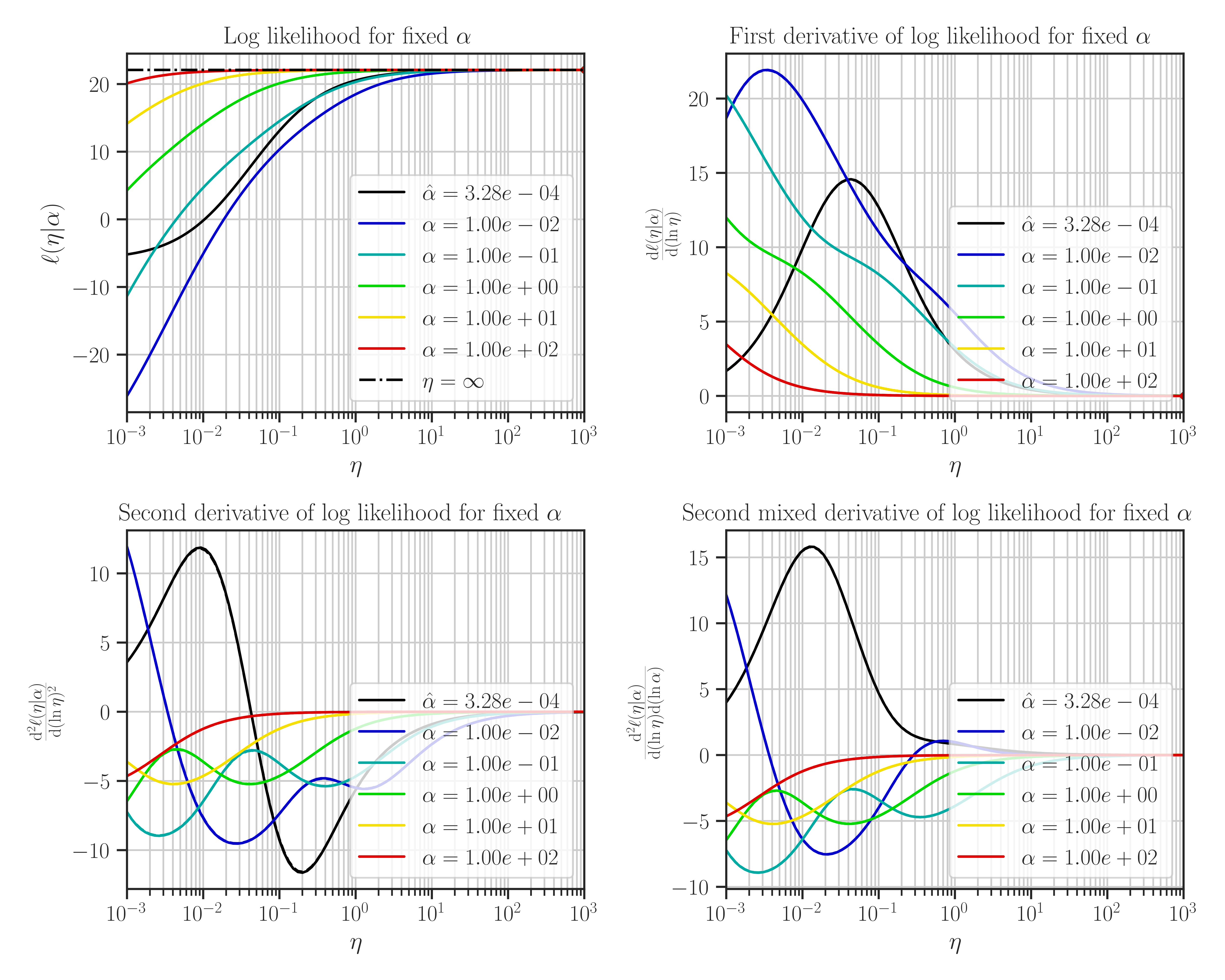
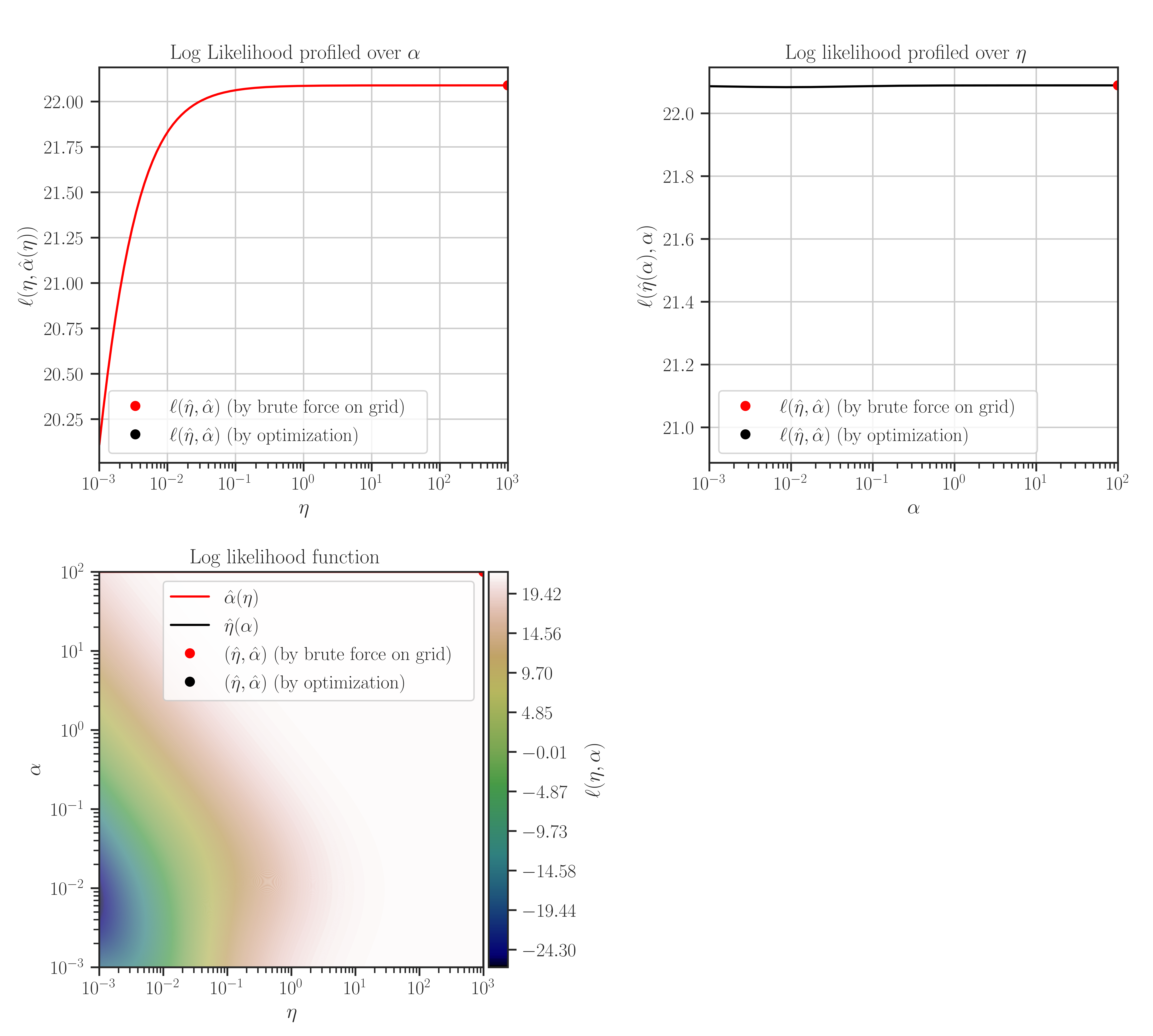
If we set profile_likelihood=none, the followings will be plotted instead: