glearn.GaussianProcess.train#
- GaussianProcess.train(z, hyperparam_guess=None, profile_hyperparam='var', log_hyperparam=True, optimization_method='Newton-CG', tol=0.001, max_iter=1000, use_rel_error=True, imate_options={}, gpu=False, verbose=False, plot=False)#
Train the hyperparameters of the Gaussian process model.
- Parameters:
- znumpy.array
An array of the size \(n\) representing the training data.
- hyperparam_guessarray_like or list, default=None
A list (or array) of the initial guess for the hyperparameters of the Gaussian process model. The unknown hyperparameters depends on the following values for the argument
profile_hyperparam:If
profile_hyperparam=none, then the hyperparameters are \([\sigma, \varsigma]\), where \(\sigma\) and \(\varsigma\) are the standard deviations of the covariance model.If
profile_hyperparam=var, then the hyperparameters are \([\eta]\), where \(\eta = \varsigma^2 / \sigma^2\).If
profile_hyperparam=var_noise, no guess is required.
If no guess for either of the parameters are given (by setting
hyperparam_guess=None), an initial guess is generated using the asymptotic analysis algorithm described in [1].- profile_hyperparam{‘none’, ‘var’, ‘var_noise’}, default: ‘var’
The type of likelihood profiling method to be used in optimization of the likelihood function.
'none': No profiling of the likelihood function. The optimization is performed in the full hyperparameter space. This is the standard method of optimizing the likelihood function.'var': The variable variable \(\sigma\) is profiled in the likelihood function. This method is the fastest. The algorithm for this method can be found in [1].'var_noise': Both variables \(\sigma\) and \(\varsigma\) are profiled in the likelihood function. The algorithm for this method can be found in [1].
- log_hyperparambool, default=True
If True, the logarithm of the hyperparameters is used during the optimization process. This allows a greater search interval of the variables, making the optimization process more efficient.
- optimization_method{‘chandrupatla’, ‘brentq’, ‘Nelder-Mead’, ‘BFGS’, ‘CG’, ‘Newton-CG’, ‘dogleg’, ‘trust-exact’, ‘trust-ncg’}, default: ‘Newton-CG’
The optimization method.
'chandrupatla': uses Jacobian only'brentq': uses Jacobian only'Nelder-Mead': uses function only (no derivative)'BFGS': uses function and Jacobian'CG': uses function and Jacobian'Newton-CG': uses function, Jacobian, and Hessian'dogleg': uses function, Jacobian, and Hessian'trust-exact': uses function, Jacobian, and Hessian'trust-ncg': uses function, Jacobian, and Hessian
In the above methods, function, Jacobian, and Hessian refers to the likelihood function and its derivatives. The Jacobian and Hessian are computed automatically and the user does not need to provide them.
- tolfloat, default: 1e-3
The tolerance of convergence of hyperparameters during optimization. In case of multiple hyperparameters, the iterations stop once the convergence criterion is satisfied for all of the hyperparameters.
- max_iterint, default: 1000
Maximum number of iterations of the optimization process.
- use_rel_errorbool or None, default=True
If True, the relative error is used for the convergence criterion. When False, the absolute error is used. When it is set to None, the callback function for minimize is not used.
- imate_optionsdict, default={}
A dictionary of options to pass arguments of the functions of the
imatepackage, such asimate.logdet(),imate.trace(), andimate.traceinv().- gpubool, default=False
If True, the computations are performed on GPU devices. Further setting on the GPU devices (such as the number of GPU devices) can be set by passing options to the
imatepackage throughimate_optionsargument.- verbosebool, default=False
If True, verbose output on the optimization process is printer both during and after the computation.
- plotbool or str, default=False
If True, the likelihood or posterior function is plotted. If
plotis a string, the plot is not shown, rather saved with a filename as the given string. If the filename does not contain file extension, the plot is saved in bothsvgandpdfformats. If the filename does not have directory path, the plot is saved in the current directory.
See also
Notes
Maximum Posterior Method:
The training process maximizes the posterior function
\[p(\boldsymbol{\beta}, \sigma, \varsigma, \boldsymbol{\alpha} \vert z) = \frac{ p(z \vert \boldsymbol{\beta}, \sigma, \varsigma, \boldsymbol{\alpha}) p(\boldsymbol{\beta}, \sigma, \varsigma, \boldsymbol{\alpha}) }{p(z)}.\]The above hyperparameters are explained in the next section below.
It is assumed that the hyperparameters are independent, namely
\[p(\boldsymbol{\beta}, \sigma, \varsigma, \boldsymbol{\alpha}) = p(\boldsymbol{\beta}) p(\sigma) p(\varsigma) p(\boldsymbol{\alpha})\]Also, it is assumed that \(p(\sigma) = 1\) and \(p(\varsigma) = 1\).
Unknown Hyperparameters:
The unknown hyperparameters are as follows:
\(\boldsymbol{\beta}\) from the linear model. A normal prior \(\boldsymbol{\beta} \sim \mathcal{N}(\boldsymbol{b}, \mathbf{B})\) for this hyperparameter can be set though
glearn.LinearModel. Once the model is trained, the optimal value of the posterior \(\hat{\boldsymbol{\beta}} \sim \mathcal{N}(\bar{\boldsymbol{\beta}},\mathbf{C})\) with the posterior mean and posterior covariance of this hyperparameter can be obtained byGaussianProcess.mean.betaandGaussianProcess.mean.Cattributes.\(\boldsymbol{\alpha} = (\alpha_1, \dots, \alpha_d)\), where \(d\) is the dimension of the space. A prior \(p(\boldsymbol{\alpha})\) or an initial guess for this hyperparameter can be set by the argument
scaleinglearn.Covarianceclass. The posterior value \(\hat{\boldsymbol{\alpha}}\) of this hyperparameter can be accessed byglearn.Covariance.get_scale()function on the attributeGaussianProcess.covcovariance object.\(\sigma\) and \(\varsigma\), which an initial guess for these hyperparameters can be set by
hyperparam_guessargument to theglearn.GaussianProcess.train()function. The optimal estimated values \(\hat{\sigma}\) and \(\hat{\varsigma}\) of these hyperparameters can be found by theglearn.Covariance.get_sigmas()function on theGaussianProcess.covattribute.
Profile Likelihood:
The profile likelihood reduces the dimension of the space of the unknown hyperparameters.
When
profile_likelihoodis set tonone, the likelihood function explicitly depends on the two hyperparameters \(\sigma\) and \(\varsigma\).When
profile_likelihoodis set tovar, the likelihood function depends on the two hyperparameters \(\eta=\varsigma^2/\sigma^2\), which is profiles over the hyperparameter \(\sigma\), reducing the number of the hyperparameters by one.When
profile_likelihoodis set tovar_sigma, the likelihood function is profiles over both \(\sigma\) and \(\eta\), reducing the number of unknown hyperparameters by two.
References
[1] (1,2,3)Ameli, S., and Shadden. S. C. (2022). Noise Estimation in Gaussian Process Regression. arXiv: 2206.09976 [cs.LG].
Examples
To define a Gaussian process object \(\mathcal{GP}(\mu, \Sigma)\), first, an object for the linear model where \(\mu\) and an object for the covariance model \(\Sigma\) should be created as follows.
1. Generate Sample Training Data:
>>> import glearn
>>> from glearn import sample_data

>>> # Generate a set of training points
>>> x = sample_data.generate_points(
...     num_points=30, dimension=1, grid=False,a=0.4, b=0.6,
...     contrast=0.9, seed=42)

>>> # Generate noise sample data on the training points
>>> y_noisy = glearn.sample_data.generate_data(
...     x, noise_magnitude=0.1)
2. Create Linear Model:
Create an object for \(\mu\) function using
glearn.LinearModelclass. On training points, the mean function is represented by the array\[\boldsymbol{\mu} = \boldsymbol{\phi}^{\intercal} (\boldsymbol{x}) \boldsymbol{\beta}.\]>>> # Create mean object using glearn. >>> mean = glearn.LinearModel(x, polynomial_degree=2)
3. Create Covariance Object:
Create the covariance model using
glearn.Covarianceclass. On the training points, the covariance function is represented by the matrix\[\boldsymbol{\Sigma}(\sigma, \varsigma, \boldsymbol{\alpha}) = \sigma^2 \mathbf{K}(\boldsymbol{\alpha}) + \varsigma^2 \mathbf{I}.\]>>> # Define a Cauchy prior for scale hyperparameter >>> scale = glearn.priors.Cauchy() >>> # Create a covariance object >>> cov = glearn.Covariance(x, scale=scale)
4. Create Gaussian Process Object:
Putting all together, we can create an object for \(\mathcal{GP} (\mu, \Sigma)\) as follows:
>>> # Gaussian process object
>>> gp = glearn.GaussianProcess(mean, cov)
5. Train The Model:
Train the model to find the regression parameter \(\boldsymbol{\beta}\) and the hyperparameters \(\sigma\), \(\varsigma\), and \(\boldsymbol{\alpha}\).
>>> # Train
>>> result = gp.train(
...     y_noisy, profile_hyperparam='var', log_hyperparam=True,
...     hyperparam_guess=None, optimization_method='Newton-CG',
...     tol=1e-2, max_iter=1000, use_rel_error=True,
...     imate_options={'method': 'cholesky'}, verbose=True)
The results of training process can be found in the
training_resultattribute as follows:>>> # Training results >>> gp.training_results { 'config': { 'max_bracket_trials': 6, 'max_iter': 1000, 'optimization_method': 'Newton-CG', 'profile_hyperparam': 'var', 'tol': 0.001, 'use_rel_error': True }, 'convergence': { 'converged': array([ True, True]), 'errors': array([[ inf, inf], [0.71584751, 0.71404119], ... [0.09390544, 0.07001806], [0. , 0. ]]), 'hyperparams': array([[-0.39474532, 0.39496465], [-0.11216787, 0.67698568], ... [ 2.52949461, 3.31844015], [ 2.52949461, 3.31844015]]) }, 'data': { 'avg_row_nnz': 30.0, 'density': 1.0, 'dimension': 1, 'kernel_threshold': None, 'nnz': 900, 'size': 30, 'sparse': False }, 'device': {}, 'hyperparam': { 'eq_sigma': 0.0509670753735289, 'eta': 338.4500691178316, 'scale': array([2081.80547198]), 'sigma': 0.002766315834132389, 'sigma0': 0.05089194699396757 }, 'imate_config': { 'device': { 'num_cpu_threads': 8, 'num_gpu_devices': 0, 'num_gpu_multiprocessors': 0, 'num_gpu_threads_per_multiprocessor': 0 }, 'imate_interpolate': False, 'imate_method': 'cholesky', 'imate_tol': 1e-08, 'max_num_samples': 0, 'min_num_samples': 0, 'solver': { 'cholmod_used': False, 'method': 'cholesky', 'version': '0.18.2' } }, 'optimization': { 'max_fun': 42.062003754316756, 'message': 'Optimization terminated successfully.', 'num_cor_eval': 45, 'num_fun_eval': 15, 'num_hes_eval': 15, 'num_jac_eval': 15, 'num_opt_iter': 15 }, 'time': { 'cor_count': 45, 'cor_proc_time': 5.494710099000002, 'cor_wall_time': 0.7112228870391846, 'det_count': 15, 'det_proc_time': 0.013328177999998747, 'det_wall_time': 0.002137899398803711, 'lik_count': 45, 'lik_proc_time': 6.337607392999995, 'lik_wall_time': 0.8268890380859375, 'opt_proc_time': 6.542538159, 'opt_wall_time': 0.8506159782409668, 'sol_count': 105, 'sol_proc_time': 1.9085943260000005, 'sol_wall_time': 0.24165892601013184, 'trc_count': 30, 'trc_proc_time': 0.05656320299999962, 'trc_wall_time': 0.006264448165893555 } }
Verbose Output:
By setting
verboseto True, useful info about the process is printed.Error ========================= itr param 1 param 2 --- -------- -------- 001 inf inf 002 6.94e+00 8.28e-01 003 7.86e-01 4.14e-01 004 4.21e-01 3.02e-01 005 2.81e-01 2.44e-01 006 2.05e-01 2.05e-01 007 1.59e-01 2.05e-01 008 1.14e-01 3.02e-01 009 8.53e-02 7.04e-02 010 7.29e-02 7.03e-02 011 6.62e-02 6.16e-02 012 6.74e-02 5.09e-02 013 6.80e-02 4.48e-02 014 0.00e+00 0.00e+00 Training Summary ================================================================================ posterior/param optimization imate solver ----------------------------- ------------------- -------------------- posterior +2.094444496e+01 method Newton-CG method cholesky eta 1.5971145695e+06 tol 1.00e-02 tol 1.00e-08 sigma 8.7512674550e-05 max iter 1000 interpolate False sigma0 1.1059589121e-01 max bracket try 6 min num samples 0 alpha 3.2828647028e-04 profile param var max num samples 0 Process ================================================================================ time (sec) evaluations processor ----------------------------- ------------------- -------------------- task clock process task # device # ================================================================================ correlation 5.83e-1 4.51e+0 correlation 42 cpu threads 8 logdet 2.12e-3 1.49e-2 likelihood 14 gpu devices 0 traceinv 5.96e-3 4.95e-2 jacobian 14 gpu multiproc 0 solver 2.09e-1 1.58e+0 hessian 14 gpu thrds/sm 0 overall 7.14e-1 5.49e+0 optimization 14 mem used (b) 2199552
Obtaining the Optimal Hyperparameter:
Once the model is trained, the optimal regression parameter \(\boldsymbol{\beta}\) of the mean function, the variance hyperparameters \(\sigma\) and \(\varsigma\) of the covariance, and the scale hyperparameters \(\boldsymbol{\alpha}\) of the covariance can be accessed as follows.
>>> # Getting beta
>>> gp.mean.beta
[ 0.07843029  3.75650903 -3.68907446]

>>> # Getting variances sigma and varsigma
>>> gp.cov.get_sigmas()
(8.751267455041524e-05, 0.11059589121331345)

>>> # Getting the scale parameter alpha
gp.cov.get_scale()
[0.00032829]
Plotting:
Plotting the convergence of the hyperparameters:
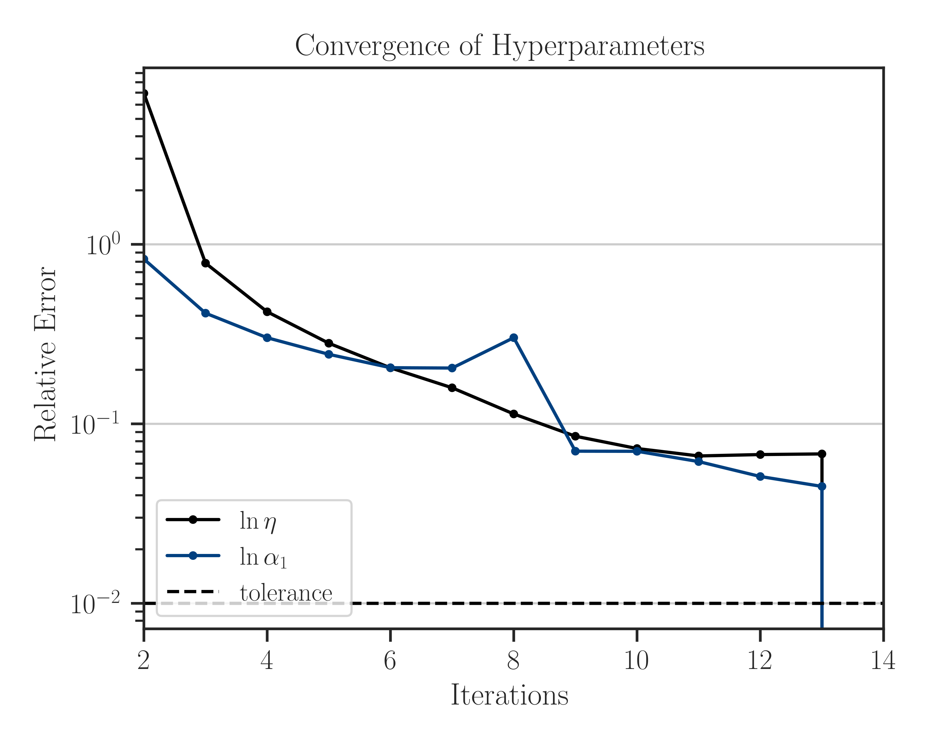
>>> # Train
>>> result = gp.train(
...     y_noisy, profile_hyperparam='var', log_hyperparam=True,
...     hyperparam_guess=None, optimization_method='Newton-CG',
...     tol=1e-6, max_iter=1000, use_rel_error=True,
...     imate_options={'method': 'cholesky'}, verbose=True,
...     plot=True)
Note that since we set
log_hyperparam=True, the logarithm of the scale hyperparameter, \(\log \alpha_1\), is used in the optimization process, as can be seen in the legend of the figure. Also, the iterations stop once the convergence error reaches the specified tolerancetol=1e-2.Passing Initial Guess for Hyperparameters:
One can set an initial guess for hyperparameters by passing the argument
hyperparam_guess. Since in the above example, the argumentprofile_hyperparamis set tovar, the unknown hyperparameters are\[(\eta, \alpha_1, \dots, \alpha_d),\]where \(d\) is the dimension of the space, here \(d=1\). Suppose we guess \(\sigma=0.1\), \(\varsigma=1\), which makes \(\eta = \varsigma^2/\sigma^2 = 100\). We also set an initial guess \(\alpha_1 = 1\) for the scale hyperparameter.
>>> # Train
>>> hyperparam_guess = [100, 0.5]
>>> result = gp.train(
...     y_noisy, profile_hyperparam='var',
...     hyperparam_guess=hyperparam_guess)

>>> # Getting variances sigma and varsigma
>>> gp.cov.get_sigmas()
(8.053463077699365e-05, 0.11059589693864141)
Using Other Profile Likelihood Methods:
Here we use no profiling method (
profile_likelihood=none) and we pass the hyperparameter guesses \((\sigma, \varsigma) = (0.1, 1, 0.5)\).>>> # Train >>> hyperparam_guess = [0.1, 1, 0.5] >>> result = gp.train( ... y_noisy, profile_hyperparam='none', ... hyperparam_guess=hyperparam_guess) >>> # Getting variances sigma and varsigma >>> gp.cov.get_sigmas() (0.0956820228647455, 0.11062417694050758)