glearn.GaussianProcess.predict#
- GaussianProcess.predict(test_points, cov=False, plot=False, true_data=None, confidence_level=0.95, verbose=False)#
Make prediction on test points.
Note
This function should be called after training the model with
glearn.GaussianProcess.train().- Parameters:
- test_pointsnumpy.array
An array of the size \(n^{\ast} \times d\) representing the coordinates of \(n^{\ast}\) training points in the \(d\) dimensional space. Each row of this array is the coordinate of a test point.
- covbool, default=False
If True, the prediction includes both the posterior mean and posterior covariance. If False, only the posterior mean is computed. Note that obtaining posterior covariance is computationally expensive, so if it is not needed, set this argument to False.
- plotbool or str, default=False
If True, the prediction result is plotted. If
plotis a string, the plot is not shown, rather saved with a filename as the given string. If the filename does not contain file extension, the plot is saved in bothsvgandpdfformats. If the filename does not have directory path, the plot is saved in the current directory.- true_datanumpy.array, default=None
An array of the size \(n^{\ast}\) of the true values of the test points data (if known). This option is used for benchmarking purposes only to compare the prediction results with their true values if known. If
plotis set to True, the true values together with the error of the prediction with respect to the true data is also plotted.- confidence_levelfloat, default=0.95
The confidence level that determines the confidence interval of the error of the prediction.
- verbosebool, default=False
If True, it prints information about the result.
See also
Notes
Consider the Gaussian process prior on the function \(y(x)\) by
\[y \sim \mathcal{GP}(\mu, \Sigma).\]This means that on the training points \(\boldsymbol{x}\), the array of training data \(\boldsymbol{y}\) has the normal distribution
\[\boldsymbol{y} \sim \mathcal{N}(\boldsymbol{\mu}, \boldsymbol{\Sigma}),\]where \(\boldsymbol{\mu}\) is the array of the mean and \(\boldsymbol{\Sigma}\) is the covariance matrix of the training points.
On some test points \(\boldsymbol{x}^{\ast}\), the posterior predictive distribution of the prediction \(\boldsymbol{y}^{\ast}(\boldsymbol{x}^{\ast})\) has the distribution
\[\boldsymbol{y}^{\ast}(\boldsymbol{x}^{\ast}) \sim \mathcal{N} \left(\boldsymbol{\mu}^{\ast}(\boldsymbol{x}^{\ast}), \mathbf{\Sigma}^{\ast \ast} (\boldsymbol{x}^{\ast}, \boldsymbol{x}'^{\ast})\right.\]where:
\(\boldsymbol{\mu}^{\ast}\) is the posterior predictive mean.
\(\mathbf{\Sigma}^{\ast \ast}\) is the posterior predictive covariance between test points and themselves.
This function finds \(\boldsymbol{\mu}^{\ast}\) and \(\boldsymbol{\Sigma}^{\ast \ast}\).
Computational Complexity:
The first call to
glearn.GaussianProcess.predict()has the computational complexity of \(\mathcal{O}((n^3 + n^{\ast})\), where \(n\) is the number of training points and \(n^{\ast}\) is the number of test points.After the first call to this function, all coefficients during the computations that are independent of the test points are stored in the Gaussian process object, which can be reused for the future calls. The computational complexity of the future calls to this function is as follows.
If posterior covariance is computed (by setting
cov=True), the computational complexity is still the same as the first call to the prediction function, namely, \(\mathcal{O}(n^3 + n^{\ast})\).If posterior covariance is not computed (by setting
cov=False), the computational complexity is \(\mathcal{O}(n^{\ast})\). See this point in the example below.
Examples
To define a Gaussian process object \(\mathcal{GP}(\mu, \Sigma)\), first, an object for the linear model where \(\mu\) and an object for the covariance model \(\Sigma\) should be created as follows.
1. Generate Sample Training Data:
>>> import glearn
>>> from glearn import sample_data

>>> # Generate a set of training points
>>> x = sample_data.generate_points(
...     num_points=30, dimension=1, grid=False,a=0.4, b=0.6,
...     contrast=0.9, seed=42)

>>> # Generate noise sample data on the training points
>>> y_noisy = glearn.sample_data.generate_data(
...     x, noise_magnitude=0.1)
2. Create Linear Model:
Create an object for \(\mu\) function using
glearn.LinearModelclass. On training points, the mean function is represented by the array\[\boldsymbol{\mu} = \boldsymbol{\phi}^{\intercal} (\boldsymbol{x}) \boldsymbol{\beta}.\]>>> # Create mean object using glearn. >>> mean = glearn.LinearModel(x, polynomial_degree=2)
3. Create Covariance Object:
Create the covariance model using
glearn.Covarianceclass. On the training points, the covariance function is represented by the matrix\[\boldsymbol{\Sigma}(\sigma, \varsigma, \boldsymbol{\alpha}) = \sigma^2 \mathbf{K}(\boldsymbol{\alpha}) + \varsigma^2 \mathbf{I}.\]>>> # Define a Cauchy prior for scale hyperparameter >>> scale = glearn.priors.Cauchy() >>> # Create a covariance object >>> cov = glearn.Covariance(x, scale=scale)
4. Create Gaussian Process Object:
Putting all together, we can create an object for \(\mathcal{GP} (\mu, \Sigma)\) as follows:
>>> # Gaussian process object
>>> gp = glearn.GaussianProcess(mean, cov)
5. Train The Model:
Train the model to find the regression parameter \(\boldsymbol{\beta}\) and the hyperparameters \(\sigma\), \(\varsigma\), and \(\boldsymbol{\alpha}\).
>>> # Train
>>> result = gp.train(y_noisy)
6. Predict on Test Points:
After training the hyperparameters, the
gpobject is ready to predict the data on new points. First, we create a set of \(1000\) test points \(\boldsymbol{x}^{\ast}\) equally distanced in the interval \([0, 1]\).>>> # Generate test points >>> test_points = sample_data.generate_points(num_points=1000, ... dimension=1, grid=True)
For the purpose of comparison, we also generate the noise-free data on the test points, \(y(\boldsymbol{x}^{\ast})\), using zero noise \(\varsigma = 0\).
>>> # True data (without noise)
>>> y_true = sample_data.generate_data(test_points,
...     noise_magnitude=0.0)
Note that the above step is unnecessary and only used for the purpose of comparison with the prediction since we already know the exact function that generated the noisy data \(y\) in the first place.
>>> # Prediction on test points
>>> y_star_mean, y_star_cov = gp.predict(
...     test_points, cov=True, plot=True, confidence_level=0.95,
...     true_data=y_true, verbose=True)
Some information about the prediction process can be found by
prediction_resultattribute ofGaussianProcessclass as follows:>>> # Prediction result >>> gp.prediction_result { 'config': { 'cov': True, 'num_test_points': 1000, 'num_training_points': 30 }, 'process': { 'memory': [24768512, 'b'], 'proc_time': 0.9903236419999999, 'wall_time': 0.13731884956359863 } }
Verbose Output:
By setting
verboseto True, useful info about the process is printed.Prediction Summary ================================================================================ process config ------------------------------------- ------------------------------------- wall time (sec) 1.08e-1 num training points 30 proc time (sec) 8.08e-1 num test points 1000 memory used (b) 23334912 compute covariance True
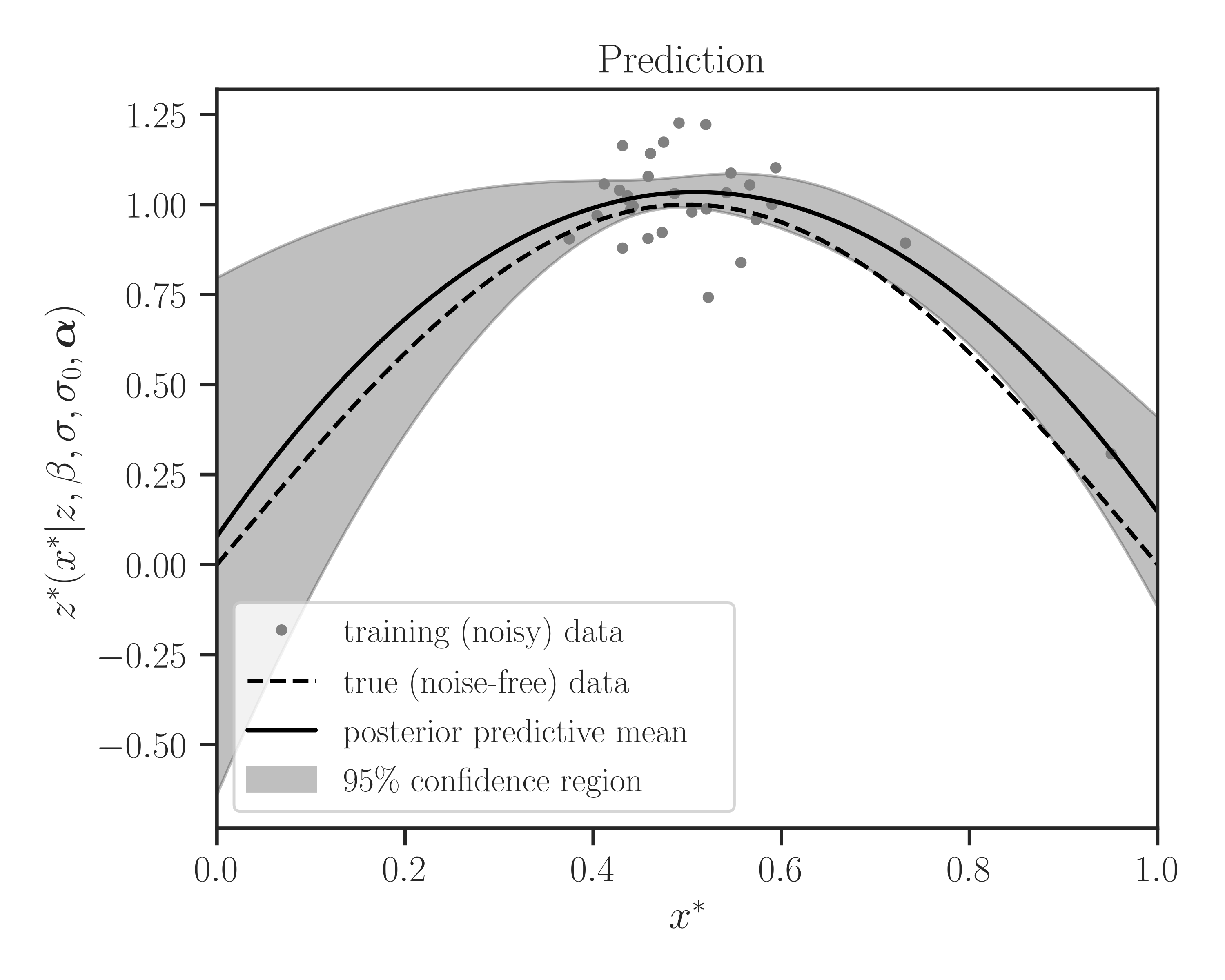
Plotting:
By setting
plotto True, the prediction is plotted as follows.>>> # Prediction on test points >>> y_star_mean, y_star_cov = gp.predict( ... test_points, cov=True, plot=True, confidence_level=0.95, ... true_data=y_true, Plot=True)
Further Call to Prediction Function:
One of the features of this function is that, once a prediction on a set of test points is made, a second and further call to this prediction function consumes significantly less processing time, provided that we only compute the posterior mean (and not the posterior covariance). This result holds even if the future alls are on a different set of test points.
To see this, let print the process time on the previous prediction:
>>> # Process time and time
>>> gp.prediction_result['process']['proc_time']
0.9903236419999999
Now, we made prediction on a different set of test points generated randomly and measure the process time:
>>> # Generate test points
>>> test_points_2 = sample_data.generate_points(num_points=1000,
...     dimension=1, grid=False)

>>> # Predict posterior mean on the new set of test points
>>> y_star_mean_2 = gp.predict(test_points_2, cov=False)

>>> # Measure the process time
>>> gp.prediction_result['process']['proc_time']
0.051906865999999496
The above process time is significantly less than the first call to the prediction function. This is because the first call to the prediction function computes the prediction coefficients that are independent of the test points. A future call to the prediction function reuses the coefficients and makes the prediction at \(\mathcal{O}(n^{\ast})\) time.